Solutions
Contents
Solutions#
Example solutions for challenge exercises from each chapter in this book.
Chapter 1 - Exercises#
You will find challenge exercises to work on at the end of each chapter. They will require you to write code such as that found in the cell at the top of this notebook.
Click the “Colab” badge at the top of this notebook to open it in the Colaboratory environment. Press
shiftandentersimultaneously on your keyboard to run the code and draw your lucky card!
Remember: Press
shiftandenteron your keyboard to run a cell.
# import necessary librarys to make the code work
import random
import calendar
from datetime import date, datetime
# define the deck and suits as character strings and split them on the spaces
deck = 'ace two three four five six seven eight nine ten jack queen king'.split()
suit = 'spades clubs hearts diamonds'.split()
print(deck)
print(suit)
['ace', 'two', 'three', 'four', 'five', 'six', 'seven', 'eight', 'nine', 'ten', 'jack', 'queen', 'king']
['spades', 'clubs', 'hearts', 'diamonds']
# define today's day and date
today = calendar.day_name[date.today().weekday()]
date = datetime.today().strftime('%Y-%m-%d')
print(today)
print(date)
Saturday
2022-10-29
# randomly sample the card value and suit
select_value = random.sample(deck, 1)[0]
select_suit = random.sample(suit, 1)[0]
print(select_value)
print(select_suit)
jack
diamonds
# combine the character strings and variables into the final statement
print("\nWelcome to TAML at SSDS!")
print("\nYour lucky card for " + today + " " + date + " is: " + select_value + " of " + select_suit)
Welcome to TAML at SSDS!

Your lucky card for Saturday 2022-10-29 is: jack of diamonds
Chapter 2 - Exercises#
(Required) Set up your Google Colaboratory (Colab) environment following the instructions in #1 listed above.
(Optional) Check that you can correctly open these notebooks in Jupyter Lab.
(Optional) Install Python Anaconda distribution on your machine.
See 2_Python_environments.ipynb for instructions.
Chapter 3 - Exercises#
Define one variablez for each of the four data types introduced above: 1) string, 2) boolean, 3) float, and 4) integer.
Define two lists that contain four elements each.
Define a dictionary that containts the two lists from #2 above.
Import the file “dracula.txt”. Save it in a variable named
dracImport the file “penguins.csv”. Save it in a variable named
penFigure out how to find help to export just the first 1000 characters of
dracas a .txt file named “dracula_short.txt”Figure out how to export the
pendataframe as a file named “penguins_saved.csv”
If you encounter error messages, which ones?
#1
string1 = "Hello!"
string2 = "This is a sentence."
print(string1)
print(string2)
Hello!
This is a sentence.
bool1 = True
bool2 = False
print(bool1)
print(bool2)
True
False
float1 = 3.14
float2 = 12.345
print(float1)
print(float2)
3.14
12.345
integer1 = 8
integer2 = 4356
print(integer1)
print(integer2)
8
4356
#2
list1 = [integer2, string2, float1, "My name is:"]
list2 = [3, True, "What?", string1]
print(list1)
print(list2)
[4356, 'This is a sentence.', 3.14, 'My name is:']
[3, True, 'What?', 'Hello!']
#3
dict_one = {"direction": "up",
           "code": 1234,
           "first_list": list1,
           "second_list": list2}
dict_one
{'direction': 'up',
 'code': 1234,
 'first_list': [4356, 'This is a sentence.', 3.14, 'My name is:'],
 'second_list': [3, True, 'What?', 'Hello!']}
#4
# !wget -P data/ https://raw.githubusercontent.com/EastBayEv/SSDS-TAML/main/fall2022/data/dracula.txt
drac = open("data/dracula.txt").read()
# print(drac)
#5
import pandas as pd
# !wget -P data/ https://raw.githubusercontent.com/EastBayEv/SSDS-TAML/main/fall2022/data/penguins.csv
pen = pd.read_csv("data/penguins.csv")
pen
| species | island | bill_length_mm | bill_depth_mm | flipper_length_mm | body_mass_g | sex | |
|---|---|---|---|---|---|---|---|
| 0 | Adelie | Torgersen | 39.1 | 18.7 | 181.0 | 3750.0 | MALE |
| 1 | Adelie | Torgersen | 39.5 | 17.4 | 186.0 | 3800.0 | FEMALE |
| 2 | Adelie | Torgersen | 40.3 | 18.0 | 195.0 | 3250.0 | FEMALE |
| 3 | Adelie | Torgersen | NaN | NaN | NaN | NaN | NaN |
| 4 | Adelie | Torgersen | 36.7 | 19.3 | 193.0 | 3450.0 | FEMALE |
| ... | ... | ... | ... | ... | ... | ... | ... |
| 339 | Gentoo | Biscoe | NaN | NaN | NaN | NaN | NaN |
| 340 | Gentoo | Biscoe | 46.8 | 14.3 | 215.0 | 4850.0 | FEMALE |
| 341 | Gentoo | Biscoe | 50.4 | 15.7 | 222.0 | 5750.0 | MALE |
| 342 | Gentoo | Biscoe | 45.2 | 14.8 | 212.0 | 5200.0 | FEMALE |
| 343 | Gentoo | Biscoe | 49.9 | 16.1 | 213.0 | 5400.0 | MALE |
344 rows × 7 columns
#6
# first slice the string you want to save
drac_short = drac[:1000]

# second, open in write mode and write the file to the data directory!
with open('data/dracula_short.txt', 'w', encoding='utf-8') as f:
    f.write(drac_short)
# You can also copy files from Colab to your Google Drive
# Mount your GDrive
# from google.colab import drive
# drive.mount('/content/drive')

# Copy a file from Colab to GDrive
# !cp data/dracula_short.txt /content/drive/MyDrive
#7
pen.to_csv("data/penguins_saved.csv")

# !cp data/penguins_saved.csv /content/drive/MyDrive
Chapter 4 - Exercises#
Load the file “gapminder-FiveYearData.csv” and save it in a variable named
gapPrint the column names
Compute the mean for one numeric column
Compute the mean for all numeric columns
Tabulate frequencies for the “continent” column
Compute mean lifeExp and dgpPercap by continent
Create a subset of
gapthat contains only countries with lifeExp greater than 75 and gdpPercap less than 5000.
#1
import pandas as pd
# !wget -P data/ https://raw.githubusercontent.com/EastBayEv/SSDS-TAML/main/fall2022/data/gapminder-FiveYearData.csv
gap = pd.read_csv("data/gapminder-FiveYearData.csv")
gap
| country | year | pop | continent | lifeExp | gdpPercap | |
|---|---|---|---|---|---|---|
| 0 | Afghanistan | 1952 | 8425333.0 | Asia | 28.801 | 779.445314 |
| 1 | Afghanistan | 1957 | 9240934.0 | Asia | 30.332 | 820.853030 |
| 2 | Afghanistan | 1962 | 10267083.0 | Asia | 31.997 | 853.100710 |
| 3 | Afghanistan | 1967 | 11537966.0 | Asia | 34.020 | 836.197138 |
| 4 | Afghanistan | 1972 | 13079460.0 | Asia | 36.088 | 739.981106 |
| ... | ... | ... | ... | ... | ... | ... |
| 1699 | Zimbabwe | 1987 | 9216418.0 | Africa | 62.351 | 706.157306 |
| 1700 | Zimbabwe | 1992 | 10704340.0 | Africa | 60.377 | 693.420786 |
| 1701 | Zimbabwe | 1997 | 11404948.0 | Africa | 46.809 | 792.449960 |
| 1702 | Zimbabwe | 2002 | 11926563.0 | Africa | 39.989 | 672.038623 |
| 1703 | Zimbabwe | 2007 | 12311143.0 | Africa | 43.487 | 469.709298 |
1704 rows × 6 columns
#2
gap.columns
Index(['country', 'year', 'pop', 'continent', 'lifeExp', 'gdpPercap'], dtype='object')
#3
gap["lifeExp"].mean()
59.474439366197174
# or
gap.describe()
| year | pop | lifeExp | gdpPercap | |
|---|---|---|---|---|
| count | 1704.00000 | 1.704000e+03 | 1704.000000 | 1704.000000 |
| mean | 1979.50000 | 2.960121e+07 | 59.474439 | 7215.327081 |
| std | 17.26533 | 1.061579e+08 | 12.917107 | 9857.454543 |
| min | 1952.00000 | 6.001100e+04 | 23.599000 | 241.165876 |
| 25% | 1965.75000 | 2.793664e+06 | 48.198000 | 1202.060309 |
| 50% | 1979.50000 | 7.023596e+06 | 60.712500 | 3531.846988 |
| 75% | 1993.25000 | 1.958522e+07 | 70.845500 | 9325.462346 |
| max | 2007.00000 | 1.318683e+09 | 82.603000 | 113523.132900 |
#4
print(gap.mean())
year         1.979500e+03
pop          2.960121e+07
lifeExp      5.947444e+01
gdpPercap    7.215327e+03
dtype: float64
/var/folders/9g/fhnd1v790cj5ccxlv4rcvsy40000gq/T/ipykernel_76196/1146573181.py:2: FutureWarning: Dropping of nuisance columns in DataFrame reductions (with 'numeric_only=None') is deprecated; in a future version this will raise TypeError.  Select only valid columns before calling the reduction.
  print(gap.mean())
#5
gap["continent"].value_counts()
Africa      624
Asia        396
Europe      360
Americas    300
Oceania      24
Name: continent, dtype: int64
#6
le_gdp_by_continent = gap.groupby("continent").agg(mean_le = ("lifeExp", "mean"),
                                                  mean_gdp = ("gdpPercap", "mean"))
le_gdp_by_continent
| mean_le | mean_gdp | |
|---|---|---|
| continent | ||
| Africa | 48.865330 | 2193.754578 |
| Americas | 64.658737 | 7136.110356 |
| Asia | 60.064903 | 7902.150428 |
| Europe | 71.903686 | 14469.475533 |
| Oceania | 74.326208 | 18621.609223 |
#7
gap_75_1000 = gap[(gap["lifeExp"] > 75) & (gap["gdpPercap"] < 5000)]
gap_75_1000
| country | year | pop | continent | lifeExp | gdpPercap | |
|---|---|---|---|---|---|---|
| 22 | Albania | 2002 | 3508512.0 | Europe | 75.651 | 4604.211737 |
Chapter 5 - Penguins Exercises#
Learn more about the biological and spatial characteristics of penguins!
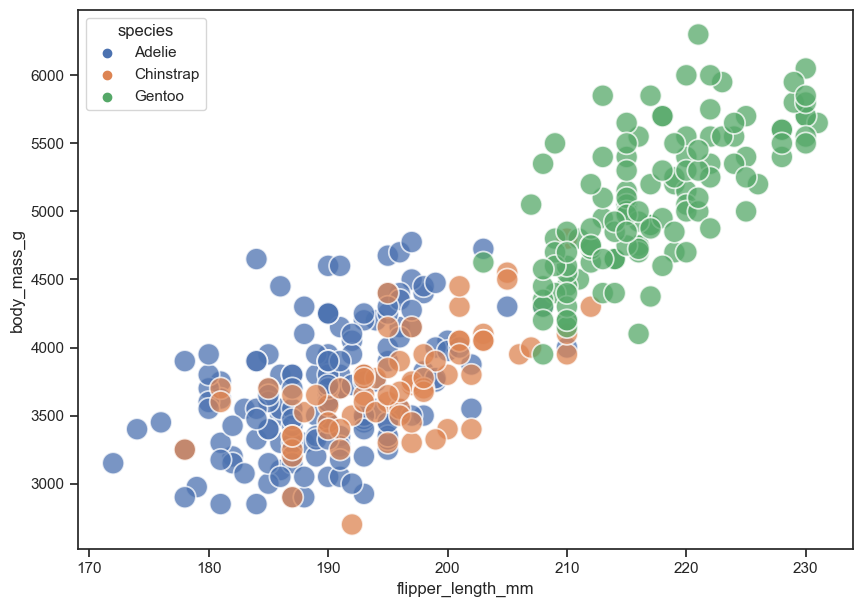
Use seaborn to make a scatterplot of two continuous variables. Color each point by species.
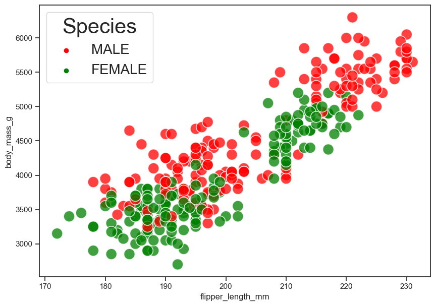
Make the same scatterplot as #1 above. This time, color each point by sex.
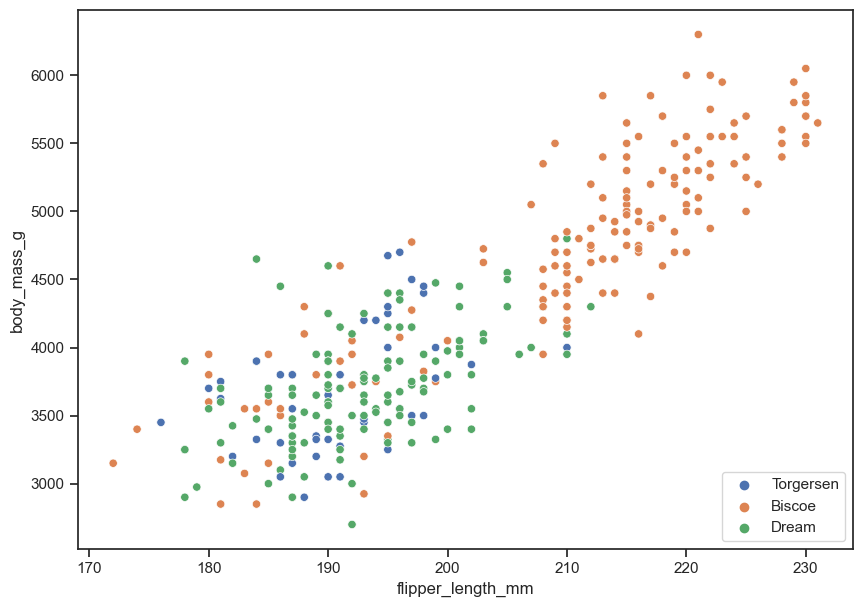
Make the same scatterplot as #1 above again. This time color each point by island.
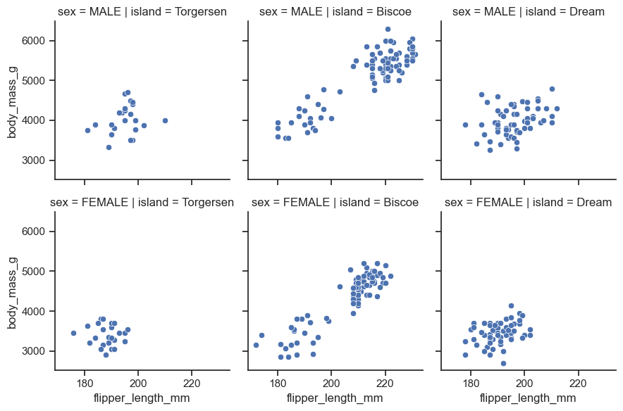
Use the
sns.FacetGridmethod to make faceted plots to examine “flipper_length_mm” on the x-axis, and “body_mass_g” on the y-axis.
import pandas as pd
import seaborn as sns
# !wget -P data/ https://raw.githubusercontent.com/EastBayEv/SSDS-TAML/main/fall2022/data/penguins.csv
peng = pd.read_csv("data/penguins.csv")
# set seaborn figure size, background theme, and axis and tick label size
sns.set(rc={'figure.figsize':(10, 7)})
sns.set(font_scale = 2)
sns.set_theme(style='ticks')
peng
| species | island | bill_length_mm | bill_depth_mm | flipper_length_mm | body_mass_g | sex | |
|---|---|---|---|---|---|---|---|
| 0 | Adelie | Torgersen | 39.1 | 18.7 | 181.0 | 3750.0 | MALE |
| 1 | Adelie | Torgersen | 39.5 | 17.4 | 186.0 | 3800.0 | FEMALE |
| 2 | Adelie | Torgersen | 40.3 | 18.0 | 195.0 | 3250.0 | FEMALE |
| 3 | Adelie | Torgersen | NaN | NaN | NaN | NaN | NaN |
| 4 | Adelie | Torgersen | 36.7 | 19.3 | 193.0 | 3450.0 | FEMALE |
| ... | ... | ... | ... | ... | ... | ... | ... |
| 339 | Gentoo | Biscoe | NaN | NaN | NaN | NaN | NaN |
| 340 | Gentoo | Biscoe | 46.8 | 14.3 | 215.0 | 4850.0 | FEMALE |
| 341 | Gentoo | Biscoe | 50.4 | 15.7 | 222.0 | 5750.0 | MALE |
| 342 | Gentoo | Biscoe | 45.2 | 14.8 | 212.0 | 5200.0 | FEMALE |
| 343 | Gentoo | Biscoe | 49.9 | 16.1 | 213.0 | 5400.0 | MALE |
344 rows × 7 columns
#1
sns.scatterplot(data = peng, x = "flipper_length_mm", y = "body_mass_g",
                hue = "species",
               s = 250, alpha = 0.75);
#2
sns.scatterplot(data = peng, x = "flipper_length_mm", y = "body_mass_g",
                hue = "sex",
               s = 250, alpha = 0.75,

               palette = ["red", "green"]).legend(title = "Species",
                                                  fontsize = 20,
                                                  title_fontsize = 30,
                                                 loc = "best");
#3
sns.scatterplot(data = peng, x = "flipper_length_mm", y = "body_mass_g",
                hue = "island").legend(loc = "lower right");
#4
facet_plot = sns.FacetGrid(data = peng, col = "island",  row = "sex")
facet_plot.map(sns.scatterplot, "flipper_length_mm", "body_mass_g");
Chapter 5 - Gapminder Exercises#
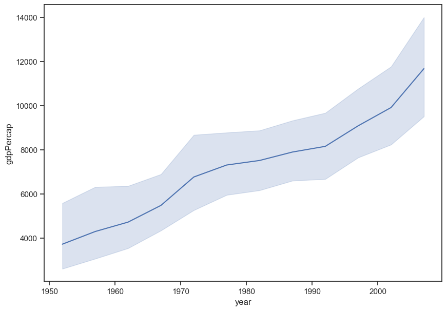
Figure out how to make a line plot that shows gdpPercap through time.
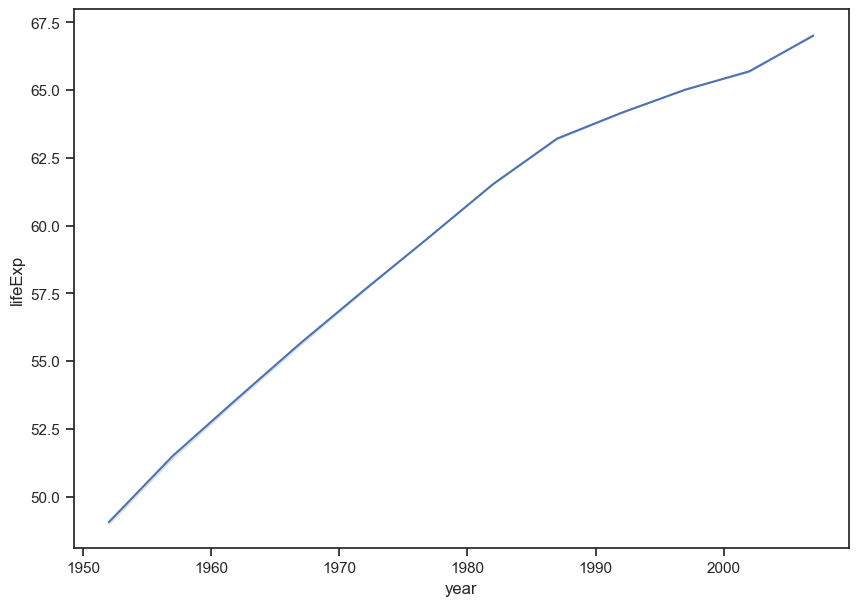
Figure out how to make a second line plot that shows lifeExp through time.
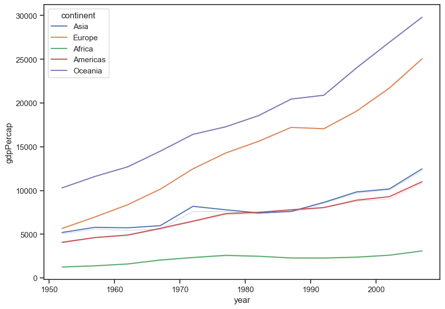
How can you plot gdpPercap with a different colored line for each continent?
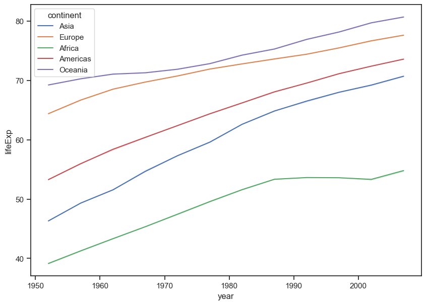
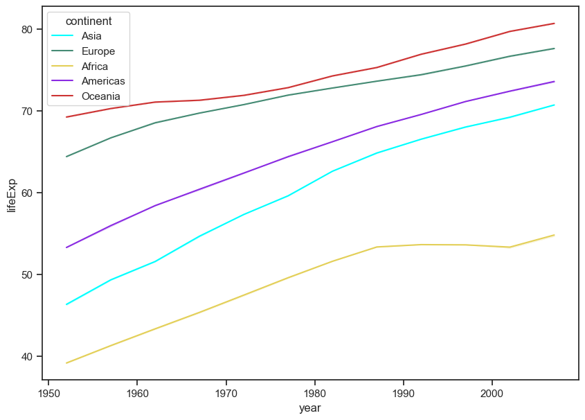
Plot lifeExp with a different colored line for each continent.
import pandas as pd
import seaborn as sns
# !wget -P data/ https://raw.githubusercontent.com/EastBayEv/SSDS-TAML/main/fall2022/data/gapminder-FiveYearData.csv
gap = pd.read_csv("data/gapminder-FiveYearData.csv")
#1
sns.lineplot(data = gap, x = "year", y = "gdpPercap", ci = 95);
#2
sns.lineplot(data = gap, x = "year", y = "lifeExp", ci = False);
#3
sns.lineplot(data = gap, x = "year", y = "gdpPercap", hue = "continent", ci = False);
#4
sns.lineplot(data = gap, x = "year", y = "lifeExp",
             hue = "continent", ci = False);
#4 with custom colors
sns.lineplot(data = gap, x = "year", y = "lifeExp",
             hue = "continent",
             ci = False,
            palette = ["#00FFFF", "#458B74", "#E3CF57", "#8A2BE2", "#CD3333"]);

# color hex codes: https://www.webucator.com/article/python-color-constants-module/
# seaborn color palettes: https://www.reddit.com/r/visualization/comments/qc0b36/all_seaborn_color_palettes_together_so_you_dont/
Exercise - scikit learn’s LinearRegression() function#
Compare our “by hand” OLS results to those producd by sklearn’s
LinearRegressionfunction. Are they the same?Slope = 4
Intercept = -4
RMSE = 2.82843
y_hat = y_hat = B0 + B1 * data.x
#1
from sklearn.linear_model import LinearRegression
from sklearn.metrics import mean_squared_error
# Recreate dataset
import pandas as pd
data = pd.DataFrame({"x": [1,2,3,4,5],
                     "y": [2,4,6,8,20]})
data
| x | y | |
|---|---|---|
| 0 | 1 | 2 |
| 1 | 2 | 4 |
| 2 | 3 | 6 |
| 3 | 4 | 8 |
| 4 | 5 | 20 |
# Our "by hand" OLS regression information:
B1 = 4
B0 = -4
RMSE = 2.82843
y_hat = B0 + B1 * data.x
# use scikit-learn to compute R-squared value
lin_mod = LinearRegression().fit(data[['x']], data[['y']])
print("R-squared: " + str(lin_mod.score(data[['x']], data[['y']])))
R-squared: 0.8
# use scikit-learn to compute slope and intercept
print("scikit-learn slope: " + str(lin_mod.coef_))
print("scikit-learn intercept: " + str(lin_mod.intercept_))
scikit-learn slope: [[4.]]
scikit-learn intercept: [-4.]
# compare to our by "hand" versions. Both are the same!
print(int(lin_mod.coef_) == B1)
print(int(lin_mod.intercept_) == B0)
True
True
# use scikit-learn to compute RMSE
RMSE_scikit = round(mean_squared_error(data.y, y_hat, squared = False), 5)
print(RMSE_scikit)
2.82843
# Does our hand-computed RMSE equal that of scikit-learn at 5 digits?? Yes!
print(round(RMSE, 5) == round(RMSE_scikit, 5))
True
Chapter 7 - Exercises - redwoods webscraping#
This also works with data scraped from the web. Below is very brief BeautifulSoup example to save the contents of the Sequoioideae (redwood trees) Wikipedia page in a variable named text.
Read through the code below
Practice by repeating for a webpage of your choice
#1
# See 7_English_preprocessing_basics.ipynb
#2
from bs4 import BeautifulSoup
import requests
import regex as re
import nltk
url = "https://en.wikipedia.org/wiki/Observable_universe"
response = requests.get(url)
soup = BeautifulSoup(response.text, 'html')
text = ""

for paragraph in soup.find_all('p'):
    text += paragraph.text
text = re.sub(r'\[[0-9]*\]',' ',text)
text = re.sub(r'\s+',' ',text)
text = re.sub(r'\d',' ',text)
text = re.sub(r'[^\w\s]','',text)
text = text.lower()
text = re.sub(r'\s+',' ',text)
# print(text)
Chapter 7 - Exercise - Dracula versus Frankenstein#
Practice your text pre-processing skills on the classic novel Dracula! Here you’ll just be performing the standardization operations on a text string instead of a DataFrame, so be sure to adapt the practices you saw with the UN HRC corpus processing appropriately.
Can you:
Remove non-alphanumeric characters & punctuation?
Remove digits?
Remove unicode characters?
Remove extraneous spaces?
Standardize casing?
Lemmatize tokens?
Investigate classic horror novel vocabulary. Create a single TF-IDF sparse matrix that contains the vocabulary for Frankenstein and Dracula. You should only have two rows (one for each of these novels), but potentially thousands of columns to represent the vocabulary across the two texts. What are the 20 most unique words in each? Make a dataframe or visualization to illustrate the differences.
Read through this 20 newsgroups dataset example to get familiar with newspaper data. Do you best to understand and explain what is happening at each step of the workflow. “The 20 newsgroups dataset comprises around 18000 newsgroups posts on 20 topics split in two subsets: one for training (or development) and the other one for testing (or for performance evaluation). The split between the train and test set is based upon a messages posted before and after a specific date.”
# 1
import regex as re
from string import punctuation
import nltk
nltk.download('stopwords')
from nltk.corpus import stopwords
import pandas as pd
from collections import Counter
import seaborn as sns
[nltk_data] Downloading package stopwords to
[nltk_data]     /Users/evanmuzzall/nltk_data...
[nltk_data]   Package stopwords is already up-to-date!
Import dracula.txt#
# !wget -P data/ https://raw.githubusercontent.com/EastBayEv/SSDS-TAML/main/fall2022/data/dracula.txt
text = open("data/dracula.txt").read()

# print just the first 100 characters
print(text[:100])
The Project Gutenberg eBook of Dracula, by Bram Stoker

This eBook is for the use of anyone anywhere
Standardize Text#
Casing and spacing#
Oftentimes in text analysis, identifying occurences of key word(s) is a necessary step. To do so, we may want “apple,” “ApPLe,” and “apple ” to be treated the same; i.e., as an occurence of the token, ‘apple.’ To achieve this, we can standardize text casing and spacing:
# Converting all charazcters in a string to lowercase only requires one method:
message = "Hello! Welcome      to        TAML!"
print(message.lower())

# To replace instances of multiple spaces with one, we can use the regex module's 'sub' function:
# Documentation on regex can be found at: https://docs.python.org/3/library/re.html
single_spaces_msg = re.sub('\s+', ' ', message)
print(single_spaces_msg)
hello! welcome      to        taml!
Hello! Welcome to TAML!
Remove punctuation#
Remember that Python methods can be chained together.
Below, a standard for loop loops through the punctuation module to replace any of these characters with nothing.
print(punctuation)
!"#$%&'()*+,-./:;<=>?@[\]^_`{|}~
for char in punctuation:
    text = text.lower().replace(char, "")
print(text[:100])
the project gutenberg ebook of dracula by bram stoker

this ebook is for the use of anyone anywhere
Tokenize the text#
Split each word on spaces.
# .split() returns a list of the tokens in a string, separated by the specified delimiter (default: " ")
tokens = text.split()
# View the first 20
print(tokens[:20])
['the', 'project', 'gutenberg', 'ebook', 'of', 'dracula', 'by', 'bram', 'stoker', 'this', 'ebook', 'is', 'for', 'the', 'use', 'of', 'anyone', 'anywhere', 'in', 'the']
Remove stop words#
Below is a list comprehension (a sort of shortcut for loop, or chunk of repeating code) that can accomplish this task for us.
filtered_text = [word for word in tokens if word not in stopwords.words('english')]
# show only the first 100 words
# do you see any stopwords?
print(filtered_text[:100])
['project', 'gutenberg', 'ebook', 'dracula', 'bram', 'stoker', 'ebook', 'use', 'anyone', 'anywhere', 'united', 'states', 'parts', 'world', 'cost', 'almost', 'restrictions', 'whatsoever', 'may', 'copy', 'give', 'away', 'reuse', 'terms', 'project', 'gutenberg', 'license', 'included', 'ebook', 'online', 'wwwgutenbergorg', 'located', 'united', 'states', 'check', 'laws', 'country', 'located', 'using', 'ebook', 'title', 'dracula', 'author', 'bram', 'stoker', 'release', 'date', 'october', '1995', 'ebook', '345', 'recently', 'updated', 'september', '5', '2022', 'language', 'english', 'produced', 'chuck', 'greif', 'online', 'distributed', 'proofreading', 'team', 'start', 'project', 'gutenberg', 'ebook', 'dracula', 'dracula', 'bram', 'stoker', 'illustration', 'colophon', 'new', 'york', 'grosset', 'dunlap', 'publishers', 'copyright', '1897', 'united', 'states', 'america', 'according', 'act', 'congress', 'bram', 'stoker', 'rights', 'reserved', 'printed', 'united', 'states', 'country', 'life', 'press', 'garden', 'city']
Lemmatizing/Stemming tokens#
Lemmatizating and stemming are related, but are different practices. Both aim to reduce the inflectional forms of a token to a common base/root. However, how they go about doing so is the key differentiating factor.
Stemming operates by removes the prefixs and/or suffixes of a word. Examples include:
flooding to flood
studies to studi
risky to risk
Lemmatization attempts to contextualize a word, arriving at it’s base meaning. Lemmatization reductions can occur across various dimensions of speech. Examples include:
Plural to singular (corpora to corpus)
Condition (better to good)
Gerund (running to run)
One technique is not strictly better than the other - it’s a matter of project needs and proper application.
stmer = nltk.PorterStemmer()

lmtzr = nltk.WordNetLemmatizer()
# do you see any differences?
token_stem  = [ stmer.stem(token) for token in filtered_text]

token_lemma = [ lmtzr.lemmatize(token) for token in filtered_text ]

print(token_stem[:20])

print(token_lemma[:20])
['project', 'gutenberg', 'ebook', 'dracula', 'bram', 'stoker', 'ebook', 'use', 'anyon', 'anywher', 'unit', 'state', 'part', 'world', 'cost', 'almost', 'restrict', 'whatsoev', 'may', 'copi']
['project', 'gutenberg', 'ebook', 'dracula', 'bram', 'stoker', 'ebook', 'use', 'anyone', 'anywhere', 'united', 'state', 'part', 'world', 'cost', 'almost', 'restriction', 'whatsoever', 'may', 'copy']
Convert to dataframe#
df = pd.DataFrame(chunked, columns=['word', 'pos'])
df.head(n = 10)
| word | pos | |
|---|---|---|
| 0 | project | NN |
| 1 | gutenberg | NN |
| 2 | ebook | NN |
| 3 | dracula | NN |
| 4 | bram | NN |
| 5 | stoker | NN |
| 6 | ebook | NN |
| 7 | use | NN |
| 8 | anyone | NN |
| 9 | anywhere | RB |
df.shape
(73541, 2)
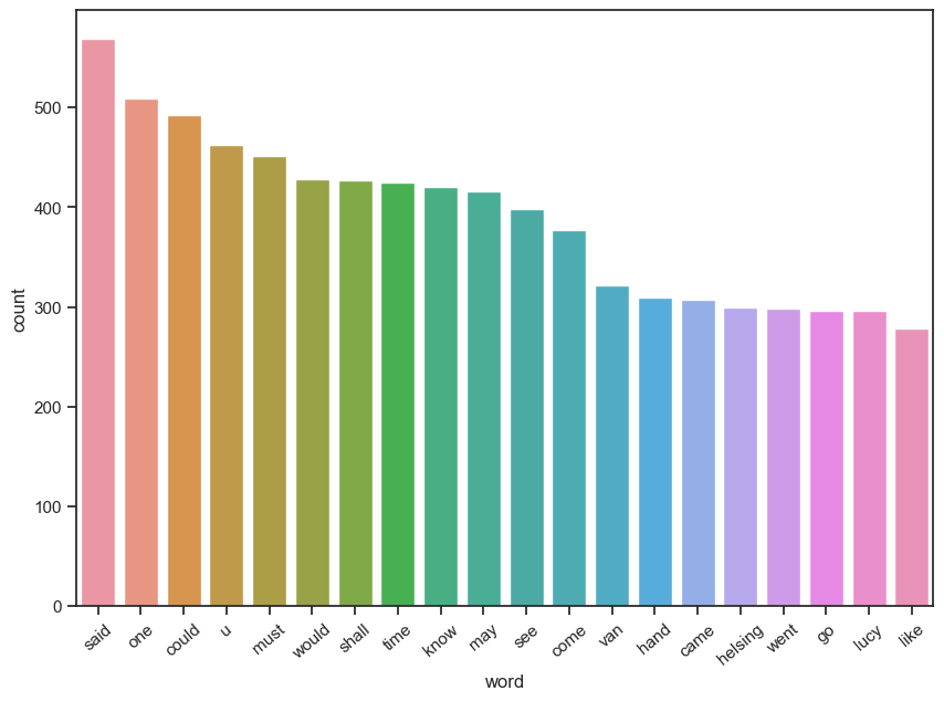
Visualize the 20 most frequent words#
top = df.copy()

count_words = Counter(top['word'])
count_words.most_common()[:20]
[('said', 569),
 ('one', 509),
 ('could', 493),
 ('u', 463),
 ('must', 451),
 ('would', 428),
 ('shall', 427),
 ('time', 425),
 ('know', 420),
 ('may', 416),
 ('see', 398),
 ('come', 377),
 ('van', 322),
 ('hand', 310),
 ('came', 307),
 ('helsing', 300),
 ('went', 298),
 ('lucy', 296),
 ('go', 296),
 ('like', 278)]
words_df = pd.DataFrame(count_words.items(), columns=['word', 'count']).sort_values(by = 'count', ascending=False)
words_df[:20]
| word | count | |
|---|---|---|
| 205 | said | 569 |
| 252 | one | 509 |
| 151 | could | 493 |
| 176 | u | 463 |
| 315 | must | 451 |
| 158 | would | 428 |
| 274 | shall | 427 |
| 161 | time | 425 |
| 220 | know | 420 |
| 17 | may | 416 |
| 378 | see | 398 |
| 680 | come | 377 |
| 120 | van | 322 |
| 1165 | hand | 310 |
| 184 | came | 307 |
| 121 | helsing | 300 |
| 542 | went | 298 |
| 155 | go | 296 |
| 100 | lucy | 296 |
| 403 | like | 278 |
# What would you need to do to improve an approach to word visualization such as this one?
top_plot = sns.barplot(x = 'word', y = 'count', data = words_df[:20])
top_plot.set_xticklabels(top_plot.get_xticklabels(),rotation = 40);
#2
import spacy
import regex as re
from sklearn.feature_extraction.text import TfidfVectorizer
---------------------------------------------------------------------------
ModuleNotFoundError                       Traceback (most recent call last)
Input In [71], in <cell line: 2>()
      1 #2
----> 2 import spacy
      3 import regex as re
      4 from sklearn.feature_extraction.text import TfidfVectorizer

ModuleNotFoundError: No module named 'spacy'
# Create a new directory to house the two novels
!mkdir data/novels/

# Download the two novels
# !wget -P data/novels/ https://raw.githubusercontent.com/EastBayEv/SSDS-TAML/main/fall2022/data/dracula.txt
# !wget -P data/novels/ https://raw.githubusercontent.com/EastBayEv/SSDS-TAML/main/fall2022/data/frankenstein.txt
mkdir: data/novels/: File exists
# See that they are there!
!ls data/novels
dracula.txt frankenstein.txt
import os
corpus = os.listdir('data/novels/')

# View the contents of this directory
corpus
['frankenstein.txt', 'dracula.txt']
empty_dictionary = {}

# Loop through the folder of documents to open and read each one
for document in corpus:
    with open('data/novels/' + document, 'r', encoding = 'utf-8') as to_open:
         empty_dictionary[document] = to_open.read()

# Populate the data frame with two columns: file name and document text
novels = (pd.DataFrame.from_dict(empty_dictionary,
                                       orient = 'index')
                .reset_index().rename(index = str,
                                      columns = {'index': 'file_name', 0: 'document_text'}))
novels
| file_name | document_text | |
|---|---|---|
| 0 | frankenstein.txt | The Project Gutenberg eBook of Frankenstein, b... |
| 1 | dracula.txt | The Project Gutenberg eBook of Dracula, by Bra... |
novels['clean_text'] = novels['document_text'].str.replace(r'[^\w\s]', ' ', regex = True)
novels
| file_name | document_text | clean_text | |
|---|---|---|---|
| 0 | frankenstein.txt | The Project Gutenberg eBook of Frankenstein, b... | The Project Gutenberg eBook of Frankenstein b... |
| 1 | dracula.txt | The Project Gutenberg eBook of Dracula, by Bra... | The Project Gutenberg eBook of Dracula by Bra... |
novels['clean_text'] = novels['clean_text'].str.replace(r'\d', ' ', regex = True)
novels
| file_name | document_text | clean_text | |
|---|---|---|---|
| 0 | frankenstein.txt | The Project Gutenberg eBook of Frankenstein, b... | The Project Gutenberg eBook of Frankenstein b... |
| 1 | dracula.txt | The Project Gutenberg eBook of Dracula, by Bra... | The Project Gutenberg eBook of Dracula by Bra... |
novels['clean_text'] = novels['clean_text'].str.encode('ascii', 'ignore').str.decode('ascii')
novels
| file_name | document_text | clean_text | |
|---|---|---|---|
| 0 | frankenstein.txt | The Project Gutenberg eBook of Frankenstein, b... | The Project Gutenberg eBook of Frankenstein b... |
| 1 | dracula.txt | The Project Gutenberg eBook of Dracula, by Bra... | The Project Gutenberg eBook of Dracula by Bra... |
novels['clean_text'] = novels['clean_text'].str.replace(r'\s+', ' ', regex = True)
novels
| file_name | document_text | clean_text | |
|---|---|---|---|
| 0 | frankenstein.txt | The Project Gutenberg eBook of Frankenstein, b... | The Project Gutenberg eBook of Frankenstein by... |
| 1 | dracula.txt | The Project Gutenberg eBook of Dracula, by Bra... | The Project Gutenberg eBook of Dracula by Bram... |
novels['clean_text'] = novels['clean_text'].str.lower()
novels
| file_name | document_text | clean_text | |
|---|---|---|---|
| 0 | frankenstein.txt | The Project Gutenberg eBook of Frankenstein, b... | the project gutenberg ebook of frankenstein by... |
| 1 | dracula.txt | The Project Gutenberg eBook of Dracula, by Bra... | the project gutenberg ebook of dracula by bram... |
# !python -m spacy download en_core_web_sm
nlp = spacy.load('en_core_web_sm')
novels['clean_text'] = novels['clean_text'].apply(lambda row: ' '.join([w.lemma_ for w in nlp(row)]))
novels
| file_name | document_text | clean_text | |
|---|---|---|---|
| 0 | frankenstein.txt | The Project Gutenberg eBook of Frankenstein, b... | the project gutenberg ebook of frankenstein by... |
| 1 | dracula.txt | The Project Gutenberg eBook of Dracula, by Bra... | the project gutenberg ebook of dracula by bram... |
tf_vectorizer = TfidfVectorizer(ngram_range = (1, 3),
                                stop_words = 'english',
                                max_df = 0.50
                                )
tf_sparse = tf_vectorizer.fit_transform(novels['clean_text'])
tf_sparse.shape
(2, 168048)
tfidf_df = pd.DataFrame(tf_sparse.todense(), columns = tf_vectorizer.get_feature_names())
tfidf_df
/Users/evanmuzzall/opt/anaconda3/lib/python3.8/site-packages/sklearn/utils/deprecation.py:87: FutureWarning: Function get_feature_names is deprecated; get_feature_names is deprecated in 1.0 and will be removed in 1.2. Please use get_feature_names_out instead.
  warnings.warn(msg, category=FutureWarning)
| aback | aback moment | aback moment know | abaft | abaft bi | abaft bi bank | abaft krok | abaft krok hooal | abandon abortion | abandon abortion spurn | ... | zophagous life eat | zophagous patient | zophagous patient effect | zophagous patient outburst | zophagous patient report | zophagous wild | zophagous wild raving | zophagy | zophagy puzzle | zophagy puzzle little | |
|---|---|---|---|---|---|---|---|---|---|---|---|---|---|---|---|---|---|---|---|---|---|
| 0 | 0.000000 | 0.000000 | 0.000000 | 0.000000 | 0.000000 | 0.000000 | 0.000000 | 0.000000 | 0.002998 | 0.002998 | ... | 0.000000 | 0.000000 | 0.000000 | 0.000000 | 0.000000 | 0.000000 | 0.000000 | 0.000000 | 0.000000 | 0.000000 |
| 1 | 0.001011 | 0.001011 | 0.001011 | 0.002021 | 0.001011 | 0.001011 | 0.001011 | 0.001011 | 0.000000 | 0.000000 | ... | 0.001011 | 0.003032 | 0.001011 | 0.001011 | 0.001011 | 0.001011 | 0.001011 | 0.001011 | 0.001011 | 0.001011 |
2 rows × 168048 columns
tfidf_df.max().sort_values(ascending = False).head(n = 20)
van            0.326435
helsing        0.310265
van helsing    0.310265
lucy           0.304201
elizabeth      0.275854
mina           0.246595
jonathan       0.210212
count          0.202127
dr             0.191010
harker         0.178882
clerval        0.176906
justine        0.164913
felix          0.149920
seward         0.140478
diary          0.120265
dr seward      0.118244
perceive       0.116938
box            0.116223
geneva         0.107943
misfortune     0.098948
dtype: float64
titles = novels['file_name'].str.slice(stop = -4)
titles = list(titles)
titles
['frankenstein', 'dracula']
tfidf_df['TITLE'] = titles
tfidf_df
| aback | aback moment | aback moment know | abaft | abaft bi | abaft bi bank | abaft krok | abaft krok hooal | abandon abortion | abandon abortion spurn | ... | zophagous patient | zophagous patient effect | zophagous patient outburst | zophagous patient report | zophagous wild | zophagous wild raving | zophagy | zophagy puzzle | zophagy puzzle little | TITLE | |
|---|---|---|---|---|---|---|---|---|---|---|---|---|---|---|---|---|---|---|---|---|---|
| 0 | 0.000000 | 0.000000 | 0.000000 | 0.000000 | 0.000000 | 0.000000 | 0.000000 | 0.000000 | 0.002998 | 0.002998 | ... | 0.000000 | 0.000000 | 0.000000 | 0.000000 | 0.000000 | 0.000000 | 0.000000 | 0.000000 | 0.000000 | frankenstein |
| 1 | 0.001011 | 0.001011 | 0.001011 | 0.002021 | 0.001011 | 0.001011 | 0.001011 | 0.001011 | 0.000000 | 0.000000 | ... | 0.003032 | 0.001011 | 0.001011 | 0.001011 | 0.001011 | 0.001011 | 0.001011 | 0.001011 | 0.001011 | dracula |
2 rows × 168049 columns
# dracula top 20 words
title = tfidf_df[tfidf_df['TITLE'] == 'frankenstein']
title.max(numeric_only = True).sort_values(ascending = False).head(20)
elizabeth                  0.275854
clerval                    0.176906
justine                    0.164913
felix                      0.149920
perceive                   0.116938
geneva                     0.107943
misfortune                 0.098948
frankenstein               0.092951
beheld                     0.083955
victor                     0.083955
murderer                   0.080957
henry                      0.077959
cousin                     0.077959
safie                      0.074960
william                    0.074960
cottager                   0.071962
chapter chapter            0.068963
chapter chapter chapter    0.065965
creator                    0.062967
exclaim                    0.059968
dtype: float64
# dracula top 20 words
title = tfidf_df[tfidf_df['TITLE'] == 'dracula']
title.max(numeric_only = True).sort_values(ascending = False).head(20)
van            0.326435
helsing        0.310265
van helsing    0.310265
lucy           0.304201
mina           0.246595
jonathan       0.210212
count          0.202127
dr             0.191010
harker         0.178882
seward         0.140478
diary          0.120265
dr seward      0.118244
box            0.116223
sort           0.096010
madam          0.095000
madam mina     0.087925
don            0.086915
quincey        0.085904
godalming      0.079840
morris         0.078829
dtype: float64
Chapter 8 - Exercise#
Read through the spacy101 guide and begin to apply its principles to your own corpus: https://spacy.io/usage/spacy-101
Chapter 9 - Exercise#
Repeat the steps in this notebook with your own data. However, real data does not come with a
fetchfunction. What importation steps do you need to consider so your own corpus works?
