Chapter 5 - Ensemble machine learning, deep learning#

2022 February 23

kandc

Texas Monthly, Music Monday: Uncovering The Mystery Of The King & Carter Jazzing Orchestra

Ensemble machine learning#

“Ensemble machine learning methods use multiple learning algorithms to obtain better predictive performance than could be obtained from any of the constituent learning algorithms.” H2O.ai ensemble example

In this manner, stacking/SuperLearner ensembles are powerful tools because they:

Eliminates bias of single algorithm selection for framing a research problem.
Allows for comparison of multiple algorithms, and/or comparison of the same model but tuned in many different ways.
Utilizes a second-level algorithm that produces an ideal weighted prediction that is suitable for data of virtually all distributions and uses external cross-validation to prevent overfitting.

The below example utilizes the h2o package, and requires Java to be installed on your machine.

install Java: https://www.java.com/en/download/help/mac_install.html
h2o SuperLearner example: https://docs.h2o.ai/h2o/latest-stable/h2o-docs/data-science/stacked-ensembles.html

Check out some other tutorials:

Python mlens library: https://mlens.readthedocs.io/en/0.1.x/install/
Machine Learning Mastery: https://machinelearningmastery.com/super-learner-ensemble-in-python/
KDNuggets: https://www.kdnuggets.com/2018/02/introduction-python-ensembles.html/2#comments

The quintessential R guide:

Guide to SuperLearner: https://cran.r-project.org/web/packages/SuperLearner/vignettes/Guide-to-SuperLearner.html

Read the papers:

H2O SuperLearner ensemble#

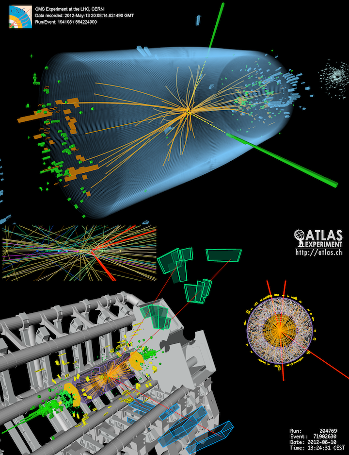
Use machine learning ensembles to detect whether or not (simulated) particle collisions produce the Higgs Boson particle or not. Learn more about the data: https://www.kaggle.com/c/higgs/overview

What is the Higgs Boson?#

“The Higgs boson is the fundamental particle associated with the Higgs field, a field that gives mass to other fundamental particles such as electrons and quarks. A particle’s mass determines how much it resists changing its speed or position when it encounters a force. Not all fundamental particles have mass. The photon, which is the particle of light and carries the electromagnetic force, has no mass at all.” (https://www.energy.gov/science/doe-explainsthe-higgs-boson)

Install h2o and Java#

# !pip install h2o

# Requires install of Java
# https://www.java.com/en/download/help/mac_install.html

Import#

import h2o
from h2o.estimators.random_forest import H2ORandomForestEstimator
from h2o.estimators.gbm import H2OGradientBoostingEstimator
from h2o.estimators.glm import H2OGeneralizedLinearEstimator
from h2o.estimators.stackedensemble import H2OStackedEnsembleEstimator
from h2o.grid.grid_search import H2OGridSearch
from __future__ import print_function

# turn off progress bars
h2o.no_progress()

---------------------------------------------------------------------------
ModuleNotFoundError                       Traceback (most recent call last)
Input In [2], in <cell line: 1>()
----> 1 import h2o
      2 from h2o.estimators.random_forest import H2ORandomForestEstimator
      3 from h2o.estimators.gbm import H2OGradientBoostingEstimator

ModuleNotFoundError: No module named 'h2o'

Initialize an h2o cluster#

h2o.init(nthreads=-1, max_mem_size='2G')

Checking whether there is an H2O instance running at http://localhost:54321 ..... not found.
Attempting to start a local H2O server...
  Java Version: java version "1.8.0_321"; Java(TM) SE Runtime Environment (build 1.8.0_321-b07); Java HotSpot(TM) 64-Bit Server VM (build 25.321-b07, mixed mode)
  Starting server from /Users/evanmuzzall/opt/anaconda3/lib/python3.8/site-packages/h2o/backend/bin/h2o.jar
  Ice root: /var/folders/9g/fhnd1v790cj5ccxlv4rcvsy40000gq/T/tmpjvise75o
  JVM stdout: /var/folders/9g/fhnd1v790cj5ccxlv4rcvsy40000gq/T/tmpjvise75o/h2o_evanmuzzall_started_from_python.out
  JVM stderr: /var/folders/9g/fhnd1v790cj5ccxlv4rcvsy40000gq/T/tmpjvise75o/h2o_evanmuzzall_started_from_python.err
  Server is running at http://127.0.0.1:54321
Connecting to H2O server at http://127.0.0.1:54321 ... successful.
Warning: Your H2O cluster version is too old (5 months and 9 days)!Please download and install the latest version from http://h2o.ai/download/

H2O_cluster_uptime:	13 secs
H2O_cluster_timezone:	America/Los_Angeles
H2O_data_parsing_timezone:	UTC
H2O_cluster_version:	3.34.0.1
H2O_cluster_version_age:	5 months and 9 days !!!
H2O_cluster_name:	H2O_from_python_evanmuzzall_evfy3t
H2O_cluster_total_nodes:	1
H2O_cluster_free_memory:	1.778 Gb
H2O_cluster_total_cores:	0
H2O_cluster_allowed_cores:	0
H2O_cluster_status:	locked, healthy
H2O_connection_url:	http://127.0.0.1:54321
H2O_connection_proxy:	{"http": null, "https": null}
H2O_internal_security:	False
H2O_API_Extensions:	Amazon S3, XGBoost, Algos, AutoML, Core V3, TargetEncoder, Core V4
Python_version:	3.8.8 final

Import a sample binary outcome train/test set into H2O#

train = h2o.import_file("https://s3.amazonaws.com/erin-data/higgs/higgs_train_10k.csv")
test = h2o.import_file("https://s3.amazonaws.com/erin-data/higgs/higgs_test_5k.csv")

train

response	x1	x2	x3	x4	x5	x6	x7	x8	x9	x10	x11	x12	x13	x14	x15	x16	x17	x18	x19	x20	x21	x22	x23	x24	x25	x26	x27	x28
1	0.869293	-0.635082	0.22569	0.32747	-0.689993	0.754202	-0.248573	-1.09206	0	1.37499	-0.653674	0.930349	1.10744	1.1389	-1.5782	-1.04699	0	0.65793	-0.0104546	-0.0457672	3.10196	1.35376	0.979563	0.978076	0.920005	0.721657	0.988751	0.876678
1	0.907542	0.329147	0.359412	1.49797	-0.31301	1.09553	-0.557525	-1.58823	2.17308	0.812581	-0.213642	1.27101	2.21487	0.499994	-1.26143	0.732156	0	0.398701	-1.13893	-0.00081911	0	0.30222	0.833048	0.9857	0.978098	0.779732	0.992356	0.798343
1	0.798835	1.47064	-1.63597	0.453773	0.425629	1.10487	1.28232	1.38166	0	0.851737	1.54066	-0.81969	2.21487	0.99349	0.35608	-0.208778	2.54822	1.25695	1.12885	0.900461	0	0.909753	1.10833	0.985692	0.951331	0.803252	0.865924	0.780118
0	1.34438	-0.876626	0.935913	1.99205	0.882454	1.78607	-1.64678	-0.942383	0	2.42326	-0.676016	0.736159	2.21487	1.29872	-1.43074	-0.364658	0	0.745313	-0.678379	-1.36036	0	0.946652	1.0287	0.998656	0.728281	0.8692	1.02674	0.957904
1	1.10501	0.321356	1.5224	0.882808	-1.20535	0.681466	-1.07046	-0.921871	0	0.800872	1.02097	0.971407	2.21487	0.596761	-0.350273	0.631194	0	0.479999	-0.373566	0.113041	0	0.755856	1.36106	0.98661	0.838085	1.1333	0.872245	0.808487
0	1.59584	-0.607811	0.00707492	1.81845	-0.111906	0.84755	-0.566437	1.58124	2.17308	0.755421	0.64311	1.42637	0	0.921661	-1.19043	-1.61559	0	0.651114	-0.654227	-1.27434	3.10196	0.823761	0.938191	0.971758	0.789176	0.430553	0.961357	0.957818
1	0.409391	-1.88468	-1.02729	1.67245	-1.6046	1.33801	0.0554274	0.0134659	2.17308	0.509783	-1.03834	0.707862	0	0.746918	-0.358465	-1.64665	0	0.367058	0.0694965	1.37713	3.10196	0.869418	1.22208	1.00063	0.545045	0.698653	0.977314	0.828786
1	0.933895	0.62913	0.527535	0.238033	-0.966569	0.547811	-0.0594392	-1.70687	2.17308	0.941003	-2.65373	-0.15722	0	1.03037	-0.175505	0.523021	2.54822	1.37355	1.29125	-1.46745	0	0.901837	1.08367	0.979696	0.7833	0.849195	0.894356	0.774879
1	1.40514	0.536603	0.689554	1.17957	-0.110061	3.2024	-1.52696	-1.57603	0	2.93154	0.567342	-0.130033	2.21487	1.78712	0.899499	0.585151	2.54822	0.401865	-0.151202	1.16349	0	1.66707	4.03927	1.17583	1.04535	1.54297	3.53483	2.74075
1	1.17657	0.104161	1.397	0.479721	0.265513	1.13556	1.53483	-0.253291	0	1.02725	0.534316	1.18002	0	2.40566	0.0875568	-0.976534	2.54822	1.25038	0.268541	0.530334	0	0.833175	0.773968	0.98575	1.1037	0.84914	0.937104	0.812364

print(train.shape)
print(test.shape)

(10000, 29)
(5000, 29)

Identify predictors and response#

x = train.columns
y = "response"
x.remove(y)

For binary classification, response should be a factor#

train[y] = train[y].asfactor()
test[y] = test[y].asfactor()

Number of CV folds (to generate level-one data for stacking)#

nfolds = 5

How to stack#

There are a few ways to assemble a list of models to stack together:

Train individual models and put them in a list
Train a grid of models
Train several grids of models

Note: All base models must have the same cross-validation folds and the cross-validated predicted values must be kept.

1. Generate a 2-model ensemble#

Use three algorithms:

random forest
gradient boosted machine
lasso

TODO: add RF and GBM defining characteristics

TODO: show how changing hyperparamters randomly can lead to overfitting (specifically # trees)

Train and cross-validate a random forest#

rf = H2ORandomForestEstimator(ntrees = 100,
                              nfolds = nfolds,
                              fold_assignment = 'Modulo',
                              keep_cross_validation_predictions = True,
                              seed = 1)
rf.train(x = x, y = y, training_frame = train)

Model Details
=============
H2ORandomForestEstimator :  Distributed Random Forest
Model Key:  DRF_model_python_1645748177867_1


Model Summary: 

		number_of_trees	number_of_internal_trees	model_size_in_bytes	min_depth	max_depth	mean_depth	min_leaves	max_leaves	mean_leaves
0		100.0	100.0	1893916.0	20.0	20.0	20.0	1394.0	1632.0	1502.23

ModelMetricsBinomial: drf
** Reported on train data. **

MSE: 0.19950487132058212
RMSE: 0.446659681771908
LogLoss: 0.5827049508751073
Mean Per-Class Error: 0.30843686874008425
AUC: 0.7598007062584857
AUCPR: 0.7763300405428175
Gini: 0.5196014125169715

Confusion Matrix (Act/Pred) for max f1 @ threshold = 0.4104450374569011: 

		0	1	Error	Rate
0	0	2150.0	2555.0	0.543	(2555.0/4705.0)
1	1	716.0	4579.0	0.1352	(716.0/5295.0)
2	Total	2866.0	7134.0	0.3271	(3271.0/10000.0)

Maximum Metrics: Maximum metrics at their respective thresholds

	metric	threshold	value	idx
0	max f1	0.410445	0.736825	260.0
1	max f2	0.239052	0.855587	344.0
2	max f0point5	0.555540	0.715899	181.0
3	max accuracy	0.520387	0.690300	200.0
4	max precision	0.999592	1.000000	0.0
5	max recall	0.095129	1.000000	386.0
6	max specificity	0.999592	1.000000	0.0
7	max absolute_mcc	0.555540	0.384066	181.0
8	max min_per_class_accuracy	0.525615	0.689896	197.0
9	max mean_per_class_accuracy	0.555540	0.691563	181.0
10	max tns	0.999592	4705.000000	0.0
11	max fns	0.999592	5294.000000	0.0
12	max fps	0.000000	4705.000000	399.0
13	max tps	0.095129	5295.000000	386.0
14	max tnr	0.999592	1.000000	0.0
15	max fnr	0.999592	0.999811	0.0
16	max fpr	0.000000	1.000000	399.0
17	max tpr	0.095129	1.000000	386.0

Gains/Lift Table: Avg response rate: 52.95 %, avg score: 52.89 %

	group	cumulative_data_fraction	lower_threshold	lift	cumulative_lift	response_rate	score	cumulative_response_rate	cumulative_score	capture_rate	cumulative_capture_rate	gain	cumulative_gain	kolmogorov_smirnov
0	1	0.0100	0.925816	1.794145	1.794145	0.950000	0.947710	0.950000	0.947710	0.017941	0.017941	79.414542	79.414542	0.016879
1	2	0.0200	0.896792	1.850803	1.822474	0.980000	0.909486	0.965000	0.928598	0.018508	0.036449	85.080264	82.247403	0.034962
2	3	0.0300	0.875029	1.813031	1.819326	0.960000	0.885540	0.963333	0.914245	0.018130	0.054580	81.303116	81.932641	0.052242
3	4	0.0400	0.857754	1.718602	1.794145	0.910000	0.866945	0.950000	0.902420	0.017186	0.071766	71.860246	79.414542	0.067515
4	5	0.0500	0.843810	1.680831	1.771483	0.890000	0.851600	0.938000	0.892256	0.016808	0.088574	68.083097	77.148253	0.081985
5	6	0.1000	0.788384	1.582625	1.677054	0.838000	0.814850	0.888000	0.853553	0.079131	0.167705	58.262512	67.705382	0.143901
6	7	0.1500	0.745567	1.571294	1.641800	0.832000	0.766710	0.869333	0.824605	0.078565	0.246270	57.129367	64.180044	0.204612
7	8	0.2000	0.704503	1.412653	1.584514	0.748000	0.724356	0.839000	0.799543	0.070633	0.316903	41.265345	58.451369	0.248465
8	9	0.3001	0.641026	1.352755	1.507209	0.716284	0.672193	0.798067	0.757065	0.135411	0.452314	35.275489	50.720927	0.323514
9	10	0.4000	0.584336	1.206116	1.432011	0.638639	0.611509	0.758250	0.720712	0.120491	0.572805	20.611641	43.201133	0.367278
10	11	0.5000	0.529812	1.046270	1.354863	0.554000	0.556784	0.717400	0.687926	0.104627	0.677432	4.627007	35.486308	0.377113
11	12	0.6000	0.474727	0.914070	1.281398	0.484000	0.503242	0.678500	0.657146	0.091407	0.768839	-8.593012	28.139754	0.358849
12	13	0.7000	0.418589	0.857413	1.220828	0.454000	0.447953	0.646429	0.627261	0.085741	0.854580	-14.258735	22.082827	0.328544
13	14	0.8000	0.353428	0.672332	1.152266	0.356000	0.386946	0.610125	0.597222	0.067233	0.921813	-32.766761	15.226629	0.258901
14	15	0.9004	0.272727	0.504121	1.079994	0.266932	0.314339	0.571857	0.565678	0.050614	0.972427	-49.587862	7.999424	0.153086
15	16	1.0000	0.000000	0.276839	1.000000	0.146586	0.196359	0.529500	0.528894	0.027573	1.000000	-72.316082	0.000000	0.000000

ModelMetricsBinomial: drf
** Reported on cross-validation data. **

MSE: 0.1978311557213644
RMSE: 0.44478214411255806
LogLoss: 0.579741500688161
Mean Per-Class Error: 0.2998532893000535
AUC: 0.7686270909034348
AUCPR: 0.7856172822797098
Gini: 0.5372541818068697

Confusion Matrix (Act/Pred) for max f1 @ threshold = 0.42006199163332014: 

		0	1	Error	Rate
0	0	2190.0	2515.0	0.5345	(2515.0/4705.0)
1	1	681.0	4614.0	0.1286	(681.0/5295.0)
2	Total	2871.0	7129.0	0.3196	(3196.0/10000.0)

Maximum Metrics: Maximum metrics at their respective thresholds

	metric	threshold	value	idx
0	max f1	0.420062	0.742756	267.0
1	max f2	0.235011	0.855768	355.0
2	max f0point5	0.560187	0.726168	186.0
3	max accuracy	0.523067	0.698300	208.0
4	max precision	0.977268	1.000000	0.0
5	max recall	0.130235	1.000000	385.0
6	max specificity	0.977268	1.000000	0.0
7	max absolute_mcc	0.560187	0.401916	186.0
8	max min_per_class_accuracy	0.523067	0.698017	208.0
9	max mean_per_class_accuracy	0.555878	0.700147	189.0
10	max tns	0.977268	4705.000000	0.0
11	max fns	0.977268	5294.000000	0.0
12	max fps	0.020000	4705.000000	399.0
13	max tps	0.130235	5295.000000	385.0
14	max tnr	0.977268	1.000000	0.0
15	max fnr	0.977268	0.999811	0.0
16	max fpr	0.020000	1.000000	399.0
17	max tpr	0.130235	1.000000	385.0

Gains/Lift Table: Avg response rate: 52.95 %, avg score: 52.85 %

	group	cumulative_data_fraction	lower_threshold	lift	cumulative_lift	response_rate	score	cumulative_response_rate	cumulative_score	capture_rate	cumulative_capture_rate	gain	cumulative_gain	kolmogorov_smirnov
0	1	0.0100	0.889002	1.813031	1.813031	0.960000	0.914104	0.960000	0.914104	0.018130	0.018130	81.303116	81.303116	0.017280
1	2	0.0200	0.866936	1.831917	1.822474	0.970000	0.877796	0.965000	0.895950	0.018319	0.036449	83.191690	82.247403	0.034962
2	3	0.0305	0.850000	1.780656	1.808078	0.942857	0.857113	0.957377	0.882580	0.018697	0.055146	78.065561	80.807752	0.052383
3	4	0.0400	0.836352	1.749416	1.794145	0.926316	0.843201	0.950000	0.873227	0.016619	0.071766	74.941603	79.414542	0.067515
4	5	0.0500	0.823457	1.718602	1.779037	0.910000	0.829764	0.942000	0.864535	0.017186	0.088952	71.860246	77.903683	0.082788
5	6	0.1010	0.770000	1.655280	1.716546	0.876471	0.793776	0.908911	0.828805	0.084419	0.173371	65.527968	71.654559	0.153817
6	7	0.1500	0.729441	1.518568	1.651873	0.804082	0.748726	0.874667	0.802646	0.074410	0.247781	51.856777	65.187284	0.207823
7	8	0.2000	0.694800	1.431539	1.596789	0.758000	0.711801	0.845500	0.779935	0.071577	0.319358	43.153919	59.678942	0.253683
8	9	0.3000	0.636224	1.371105	1.521561	0.726000	0.665173	0.805667	0.741681	0.137110	0.456468	37.110482	52.156122	0.332558
9	10	0.4011	0.580000	1.232897	1.448801	0.652819	0.607113	0.767140	0.707762	0.124646	0.581114	23.289706	44.880144	0.382602
10	11	0.5000	0.529246	1.050269	1.369972	0.556117	0.554347	0.725400	0.677416	0.103872	0.684986	5.026873	36.997167	0.393169
11	12	0.6001	0.479333	0.915043	1.294087	0.484515	0.503495	0.685219	0.648405	0.091596	0.776582	-8.495659	29.408712	0.375094
12	13	0.7000	0.427236	0.846928	1.230271	0.448448	0.452868	0.651429	0.620499	0.084608	0.861190	-15.307186	23.027115	0.342593
13	14	0.8000	0.364682	0.632672	1.155571	0.335000	0.395935	0.611875	0.592429	0.063267	0.924457	-36.732767	15.557129	0.264521
14	15	0.9018	0.290000	0.480492	1.079365	0.254420	0.328383	0.571524	0.562622	0.048914	0.973371	-51.950815	7.936472	0.152117
15	16	1.0000	0.020000	0.271170	1.000000	0.143585	0.215219	0.529500	0.528507	0.026629	1.000000	-72.882999	0.000000	0.000000

Cross-Validation Metrics Summary:

		mean	sd	cv_1_valid	cv_2_valid	cv_3_valid	cv_4_valid	cv_5_valid
0	accuracy	0.684700	0.009686	0.688000	0.683500	0.668500	0.691000	0.692500
1	auc	0.768961	0.005747	0.777448	0.764756	0.763700	0.766779	0.772118
2	err	0.315300	0.009686	0.312000	0.316500	0.331500	0.309000	0.307500
3	err_count	630.600000	19.372662	624.000000	633.000000	663.000000	618.000000	615.000000
4	f0point5	0.686030	0.008300	0.687034	0.684970	0.677061	0.699269	0.681818
5	f1	0.744774	0.007659	0.747164	0.753601	0.741520	0.748166	0.733420
6	f2	0.814755	0.016714	0.818828	0.837515	0.819545	0.804416	0.793472
7	lift_top_group	1.815754	0.126244	1.897533	1.775701	1.760890	1.660517	1.984127
8	logloss	0.579742	0.004706	0.571577	0.581464	0.582822	0.582803	0.580041
9	max_per_class_error	0.524409	0.052263	0.520085	0.570968	0.580890	0.493450	0.456653
10	mcc	0.379194	0.021935	0.389069	0.384129	0.342742	0.379066	0.400963
11	mean_per_class_accuracy	0.672491	0.015187	0.677339	0.666853	0.650241	0.676707	0.691316
12	mean_per_class_error	0.327509	0.015187	0.322661	0.333147	0.349759	0.323293	0.308684
13	mse	0.197831	0.001922	0.194467	0.198626	0.199179	0.198811	0.198073
14	pr_auc	0.786175	0.008145	0.795368	0.780520	0.791291	0.788378	0.775318
15	precision	0.651826	0.011298	0.652051	0.645764	0.639973	0.670073	0.651270
16	r2	0.205297	0.008929	0.219856	0.201582	0.198281	0.199106	0.207659
17	recall	0.869391	0.026604	0.874763	0.904673	0.881372	0.846863	0.839286
18	rmse	0.444778	0.002167	0.440985	0.445675	0.446295	0.445882	0.445053
19	specificity	0.475591	0.052263	0.479915	0.429032	0.419110	0.506550	0.543347

Scoring History:

	timestamp	duration	number_of_trees	training_rmse	training_logloss	training_auc	training_pr_auc	training_lift	training_classification_error
0	2022-02-24 16:17:21	20.602 sec	0.0	NaN	NaN	NaN	NaN	NaN	NaN
1	2022-02-24 16:17:21	20.673 sec	1.0	0.642818	14.048395	0.577384	0.589593	1.144218	0.464917
2	2022-02-24 16:17:21	20.709 sec	2.0	0.615404	11.895281	0.595767	0.598674	1.167648	0.470126
3	2022-02-24 16:17:21	20.744 sec	3.0	0.596109	10.322973	0.606984	0.606263	1.188141	0.471944
4	2022-02-24 16:17:21	20.776 sec	4.0	0.578952	8.963477	0.617051	0.613281	1.205225	0.473260
5	2022-02-24 16:17:21	20.810 sec	5.0	0.566757	7.823122	0.621447	0.619131	1.222342	0.472650
6	2022-02-24 16:17:21	20.842 sec	6.0	0.555494	6.782681	0.625539	0.623303	1.235544	0.472576
7	2022-02-24 16:17:21	20.881 sec	7.0	0.542668	5.762143	0.634190	0.632386	1.256193	0.470778
8	2022-02-24 16:17:21	20.919 sec	8.0	0.534223	5.001247	0.637938	0.634830	1.257749	0.470999
9	2022-02-24 16:17:21	20.954 sec	9.0	0.525930	4.327270	0.643458	0.638581	1.259426	0.416980
10	2022-02-24 16:17:21	20.986 sec	10.0	0.516709	3.691988	0.652861	0.649779	1.292382	0.416650
11	2022-02-24 16:17:21	21.019 sec	11.0	0.510283	3.222738	0.659091	0.656853	1.315126	0.417606
12	2022-02-24 16:17:21	21.052 sec	12.0	0.501990	2.723957	0.669423	0.667708	1.341061	0.422262
13	2022-02-24 16:17:21	21.081 sec	13.0	0.496251	2.349060	0.675311	0.675563	1.374979	0.405793
14	2022-02-24 16:17:22	21.114 sec	14.0	0.492259	2.050819	0.679020	0.680861	1.408270	0.405386
15	2022-02-24 16:17:22	21.144 sec	15.0	0.487936	1.795128	0.684347	0.686164	1.425637	0.404943
16	2022-02-24 16:17:22	21.175 sec	16.0	0.484170	1.579896	0.689326	0.694656	1.472602	0.384615
17	2022-02-24 16:17:22	21.209 sec	17.0	0.480754	1.424860	0.693815	0.699750	1.494407	0.400180
18	2022-02-24 16:17:22	21.241 sec	18.0	0.477989	1.318464	0.698239	0.703253	1.498109	0.389139
19	2022-02-24 16:17:22	21.275 sec	19.0	0.475932	1.215350	0.701065	0.707162	1.521093	0.391439

See the whole table with table.as_data_frame()

Variable Importances: 

	variable	relative_importance	scaled_importance	percentage
0	x26	15628.322266	1.000000	0.101301
1	x28	9415.993164	0.602495	0.061034
2	x27	9318.841797	0.596279	0.060404
3	x6	7188.417969	0.459961	0.046595
4	x25	7121.043945	0.455650	0.046158
5	x23	7112.994141	0.455135	0.046106
6	x4	6268.571289	0.401103	0.040632
7	x1	5769.832031	0.369191	0.037400
8	x10	5658.928223	0.362094	0.036681
9	x2	5388.754395	0.344807	0.034929
10	x7	5388.225098	0.344773	0.034926
11	x19	5345.022461	0.342009	0.034646
12	x12	5334.650391	0.341345	0.034579
13	x5	5298.523438	0.339033	0.034345
14	x20	5295.863281	0.338863	0.034327
15	x16	5240.296387	0.335308	0.033967
16	x3	5225.997070	0.334393	0.033874
17	x8	5220.911621	0.334067	0.033842
18	x15	5183.947266	0.331702	0.033602
19	x11	5183.041504	0.331644	0.033596

See the whole table with table.as_data_frame()

Random forest test set performance#

rf.model_performance(test)

ModelMetricsBinomial: drf
** Reported on test data. **

MSE: 0.19456237288967487
RMSE: 0.4410922498635346
LogLoss: 0.5723749503451226
Mean Per-Class Error: 0.2902132075244037
AUC: 0.7786910723119803
AUCPR: 0.8019489749908004
Gini: 0.5573821446239606

Confusion Matrix (Act/Pred) for max f1 @ threshold = 0.3900028567254543: 

		0	1	Error	Rate
0	0	957.0	1358.0	0.5866	(1358.0/2315.0)
1	1	280.0	2405.0	0.1043	(280.0/2685.0)
2	Total	1237.0	3763.0	0.3276	(1638.0/5000.0)

Maximum Metrics: Maximum metrics at their respective thresholds

	metric	threshold	value	idx
0	max f1	0.390003	0.745968	280.0
1	max f2	0.252355	0.861172	348.0
2	max f0point5	0.545964	0.738321	184.0
3	max accuracy	0.503137	0.710400	211.0
4	max precision	0.976952	1.000000	0.0
5	max recall	0.145391	1.000000	382.0
6	max specificity	0.976952	1.000000	0.0
7	max absolute_mcc	0.515110	0.418565	204.0
8	max min_per_class_accuracy	0.513699	0.709125	205.0
9	max mean_per_class_accuracy	0.515110	0.709787	204.0
10	max tns	0.976952	2315.000000	0.0
11	max fns	0.976952	2684.000000	0.0
12	max fps	0.040096	2315.000000	399.0
13	max tps	0.145391	2685.000000	382.0
14	max tnr	0.976952	1.000000	0.0
15	max fnr	0.976952	0.999628	0.0
16	max fpr	0.040096	1.000000	399.0
17	max tpr	0.145391	1.000000	382.0

Gains/Lift Table: Avg response rate: 53.70 %, avg score: 52.30 %

	group	cumulative_data_fraction	lower_threshold	lift	cumulative_lift	response_rate	score	cumulative_response_rate	cumulative_score	capture_rate	cumulative_capture_rate	gain	cumulative_gain	kolmogorov_smirnov
0	1	0.0100	0.892945	1.824953	1.824953	0.980000	0.916686	0.980000	0.916686	0.018250	0.018250	82.495345	82.495345	0.017818
1	2	0.0200	0.869782	1.713222	1.769088	0.920000	0.881167	0.950000	0.898926	0.017132	0.035382	71.322160	76.908752	0.033222
2	3	0.0300	0.854788	1.713222	1.750466	0.920000	0.862835	0.940000	0.886896	0.017132	0.052514	71.322160	75.046555	0.048626
3	4	0.0400	0.840256	1.862197	1.778399	1.000000	0.847272	0.955000	0.876990	0.018622	0.071136	86.219739	77.839851	0.067248
4	5	0.0500	0.827591	1.787709	1.780261	0.960000	0.833668	0.956000	0.868325	0.017877	0.089013	78.770950	78.026071	0.084261
5	6	0.1000	0.771550	1.623836	1.702048	0.872000	0.797458	0.914000	0.832892	0.081192	0.170205	62.383613	70.204842	0.151630
6	7	0.1500	0.726679	1.646182	1.683426	0.884000	0.748252	0.904000	0.804678	0.082309	0.252514	64.618250	68.342644	0.221412
7	8	0.2012	0.690000	1.498487	1.636364	0.804688	0.706711	0.878728	0.779748	0.076723	0.329236	49.848696	63.636431	0.276537
8	9	0.3000	0.628621	1.368376	1.548107	0.734818	0.658471	0.831333	0.739808	0.135196	0.464432	36.837582	54.810677	0.355145
9	10	0.4000	0.572950	1.180633	1.456238	0.634000	0.600572	0.782000	0.704999	0.118063	0.582495	18.063315	45.623836	0.394158
10	11	0.5000	0.521722	1.083799	1.381750	0.582000	0.545898	0.742000	0.673179	0.108380	0.690875	8.379888	38.175047	0.412258
11	12	0.6000	0.469495	0.953445	1.310366	0.512000	0.494960	0.703667	0.643476	0.095345	0.786220	-4.655493	31.036623	0.402202
12	13	0.7000	0.417658	0.670391	1.218941	0.360000	0.442290	0.654571	0.614735	0.067039	0.853259	-32.960894	21.894121	0.331013
13	14	0.8010	0.360000	0.700629	1.153586	0.376238	0.389071	0.619476	0.586280	0.070764	0.924022	-29.937128	15.358595	0.265707
14	15	0.9000	0.284405	0.511634	1.082971	0.274747	0.326935	0.581556	0.557752	0.050652	0.974674	-48.836597	8.297124	0.161283
15	16	1.0000	0.040000	0.253259	1.000000	0.136000	0.209755	0.537000	0.522953	0.025326	1.000000	-74.674115	0.000000	0.000000

Train and cross-validate a gradient boosted machine#

gbm = H2OGradientBoostingEstimator(distribution = "bernoulli",
                                   ntrees = 10,
                                   max_depth = 3,
                                   min_rows = 2,
                                   learn_rate = 0.2,
                                   nfolds = nfolds,
                                   fold_assignment = "Modulo",
                                   keep_cross_validation_predictions = True,
                                   seed = 1)
gbm.train(x = x, y = y, training_frame = train)

Model Details
=============
H2OGradientBoostingEstimator :  Gradient Boosting Machine
Model Key:  GBM_model_python_1645663571276_2785


Model Summary: 

		number_of_trees	number_of_internal_trees	model_size_in_bytes	min_depth	max_depth	mean_depth	min_leaves	max_leaves	mean_leaves
0		10.0	10.0	1579.0	3.0	3.0	3.0	8.0	8.0	8.0

ModelMetricsBinomial: gbm
** Reported on train data. **

MSE: 0.20052170746266884
RMSE: 0.44779650228945383
LogLoss: 0.5879177464092424
Mean Per-Class Error: 0.29613223631461116
AUC: 0.7735466157694937
AUCPR: 0.7909110775032231
Gini: 0.5470932315389874

Confusion Matrix (Act/Pred) for max f1 @ threshold = 0.4424199442800167: 

		0	1	Error	Rate
0	0	2433.0	2272.0	0.4829	(2272.0/4705.0)
1	1	818.0	4477.0	0.1545	(818.0/5295.0)
2	Total	3251.0	6749.0	0.309	(3090.0/10000.0)

Maximum Metrics: Maximum metrics at their respective thresholds

	metric	threshold	value	idx
0	max f1	0.442420	0.743441	244.0
1	max f2	0.335831	0.858813	324.0
2	max f0point5	0.542377	0.726119	166.0
3	max accuracy	0.507400	0.704200	192.0
4	max precision	0.790473	0.973684	3.0
5	max recall	0.158255	1.000000	394.0
6	max specificity	0.803933	0.999575	0.0
7	max absolute_mcc	0.519330	0.407039	183.0
8	max min_per_class_accuracy	0.513347	0.703507	187.0
9	max mean_per_class_accuracy	0.519330	0.703868	183.0
10	max tns	0.803933	4703.000000	0.0
11	max fns	0.803933	5245.000000	0.0
12	max fps	0.116664	4705.000000	399.0
13	max tps	0.158255	5295.000000	394.0
14	max tnr	0.803933	0.999575	0.0
15	max fnr	0.803933	0.990557	0.0
16	max fpr	0.116664	1.000000	399.0
17	max tpr	0.158255	1.000000	394.0

Gains/Lift Table: Avg response rate: 52.95 %, avg score: 52.93 %

	group	cumulative_data_fraction	lower_threshold	lift	cumulative_lift	response_rate	score	cumulative_response_rate	cumulative_score	capture_rate	cumulative_capture_rate	gain	cumulative_gain	kolmogorov_smirnov
0	1	0.0165	0.788097	1.831345	1.831345	0.969697	0.794128	0.969697	0.794128	0.030217	0.030217	83.134461	83.134461	0.029154
1	2	0.0309	0.779039	1.770538	1.803008	0.937500	0.780161	0.954693	0.787619	0.025496	0.055713	77.053824	80.300766	0.052737
2	3	0.0403	0.769898	1.727844	1.785476	0.914894	0.776514	0.945409	0.785029	0.016242	0.071955	72.784441	78.547579	0.067279
3	4	0.0520	0.766379	1.662591	1.757827	0.880342	0.767629	0.930769	0.781114	0.019452	0.091407	66.259090	75.782669	0.083756
4	5	0.1019	0.733553	1.680415	1.719918	0.889780	0.746516	0.910697	0.764171	0.083853	0.175260	68.041465	71.991834	0.155919
5	6	0.1501	0.703064	1.586872	1.677195	0.840249	0.720131	0.888075	0.750029	0.076487	0.251747	58.687245	67.719474	0.216040
6	7	0.2100	0.672701	1.475547	1.619677	0.781302	0.681960	0.857619	0.730613	0.088385	0.340132	47.554706	61.967714	0.276583
7	8	0.3003	0.631813	1.294604	1.521928	0.685493	0.653431	0.805861	0.707405	0.116903	0.457035	29.460397	52.192787	0.333124
8	9	0.4003	0.582373	1.242682	1.452169	0.658000	0.607055	0.768923	0.682336	0.124268	0.581303	24.268178	45.216866	0.384704
9	10	0.5000	0.519662	1.102458	1.382436	0.583751	0.552458	0.732000	0.656438	0.109915	0.691218	10.245751	38.243626	0.406415
10	11	0.6000	0.470374	0.906516	1.303116	0.480000	0.494559	0.690000	0.629458	0.090652	0.781870	-9.348442	30.311615	0.386546
11	12	0.7004	0.436366	0.795684	1.230377	0.421315	0.451070	0.651485	0.603887	0.079887	0.861756	-20.431588	23.037746	0.342947
12	13	0.8000	0.408689	0.584017	1.149906	0.309237	0.422132	0.608875	0.581258	0.058168	0.919924	-41.598310	14.990557	0.254887
13	14	0.9009	0.350489	0.580236	1.086103	0.307235	0.385621	0.575092	0.559347	0.058546	0.978470	-41.976414	8.610307	0.164868
14	15	1.0000	0.116664	0.217253	1.000000	0.115035	0.256620	0.529500	0.529347	0.021530	1.000000	-78.274728	0.000000	0.000000

ModelMetricsBinomial: gbm
** Reported on cross-validation data. **

MSE: 0.20591759601729728
RMSE: 0.4537814408030559
LogLoss: 0.5996635025616064
Mean Per-Class Error: 0.3109957762972908
AUC: 0.752800639024444
AUCPR: 0.7705701530928649
Gini: 0.5056012780488881

Confusion Matrix (Act/Pred) for max f1 @ threshold = 0.4159392211190996: 

		0	1	Error	Rate
0	0	1696.0	3009.0	0.6395	(3009.0/4705.0)
1	1	538.0	4757.0	0.1016	(538.0/5295.0)
2	Total	2234.0	7766.0	0.3547	(3547.0/10000.0)

Maximum Metrics: Maximum metrics at their respective thresholds

	metric	threshold	value	idx
0	max f1	0.415939	0.728428	268.0
1	max f2	0.279109	0.855982	346.0
2	max f0point5	0.561962	0.711702	154.0
3	max accuracy	0.517902	0.688800	186.0
4	max precision	0.835804	1.000000	0.0
5	max recall	0.158348	1.000000	392.0
6	max specificity	0.835804	1.000000	0.0
7	max absolute_mcc	0.517902	0.377372	186.0
8	max min_per_class_accuracy	0.515693	0.687354	188.0
9	max mean_per_class_accuracy	0.519427	0.689004	185.0
10	max tns	0.835804	4705.000000	0.0
11	max fns	0.835804	5287.000000	0.0
12	max fps	0.098410	4705.000000	399.0
13	max tps	0.158348	5295.000000	392.0
14	max tnr	0.835804	1.000000	0.0
15	max fnr	0.835804	0.998489	0.0
16	max fpr	0.098410	1.000000	399.0
17	max tpr	0.158348	1.000000	392.0

Gains/Lift Table: Avg response rate: 52.95 %, avg score: 52.91 %

	group	cumulative_data_fraction	lower_threshold	lift	cumulative_lift	response_rate	score	cumulative_response_rate	cumulative_score	capture_rate	cumulative_capture_rate	gain	cumulative_gain	kolmogorov_smirnov
0	1	0.0101	0.789519	1.776382	1.776382	0.940594	0.800149	0.940594	0.800149	0.017941	0.017941	77.638160	77.638160	0.016666
1	2	0.0204	0.781367	1.815231	1.795997	0.961165	0.785390	0.950980	0.792698	0.018697	0.036638	81.523144	79.599696	0.034513
2	3	0.0335	0.778060	1.715575	1.764548	0.908397	0.779096	0.934328	0.787379	0.022474	0.059112	71.557497	76.454836	0.054436
3	4	0.0407	0.771218	1.678733	1.749367	0.888889	0.774200	0.926290	0.785047	0.012087	0.071199	67.873256	74.936719	0.064823
4	5	0.0523	0.764063	1.693204	1.736910	0.896552	0.766315	0.919694	0.780893	0.019641	0.090840	69.320439	73.691043	0.081914
5	6	0.1010	0.729840	1.609360	1.675408	0.852156	0.745647	0.887129	0.763898	0.078376	0.169216	60.935988	67.540833	0.144987
6	7	0.1501	0.699633	1.565478	1.639448	0.828921	0.716835	0.868088	0.748503	0.076865	0.246081	56.547794	63.944843	0.203998
7	8	0.2000	0.675508	1.426839	1.586402	0.755511	0.686070	0.840000	0.732926	0.071199	0.317280	42.683857	58.640227	0.249268
8	9	0.3000	0.628903	1.318225	1.497010	0.698000	0.649476	0.792667	0.705109	0.131822	0.449103	31.822474	49.700976	0.316903
9	10	0.4000	0.579228	1.218130	1.427290	0.645000	0.605317	0.755750	0.680161	0.121813	0.570916	21.813031	42.728990	0.363265
10	11	0.5000	0.520964	1.059490	1.353730	0.561000	0.550914	0.716800	0.654312	0.105949	0.676865	5.949008	35.372993	0.375909
11	12	0.6000	0.470755	0.900850	1.278250	0.477000	0.494393	0.676833	0.627659	0.090085	0.766950	-9.915014	27.824992	0.354835
12	13	0.7009	0.438080	0.758050	1.203363	0.401388	0.452376	0.637181	0.602425	0.076487	0.843437	-24.194993	20.336311	0.302948
13	14	0.8003	0.407245	0.714390	1.142631	0.378270	0.423648	0.605023	0.580221	0.071010	0.914448	-28.560979	14.263100	0.242609
14	15	0.9001	0.350168	0.580954	1.080354	0.307615	0.382479	0.572048	0.558296	0.057979	0.972427	-41.904583	8.035420	0.153723
15	16	1.0000	0.098410	0.276008	1.000000	0.146146	0.265874	0.529500	0.529083	0.027573	1.000000	-72.399217	0.000000	0.000000

Cross-Validation Metrics Summary:

		mean	sd	cv_1_valid	cv_2_valid	cv_3_valid	cv_4_valid	cv_5_valid
0	accuracy	0.662000	0.011028	0.660500	0.659000	0.647500	0.665000	0.678000
1	auc	0.753708	0.008455	0.767336	0.754202	0.749615	0.744636	0.752753
2	err	0.338000	0.011028	0.339500	0.341000	0.352500	0.335000	0.322000
3	err_count	676.000000	22.056746	679.000000	682.000000	705.000000	670.000000	644.000000
4	f0point5	0.667733	0.006292	0.664405	0.665501	0.660570	0.676335	0.671854
5	f1	0.732593	0.011290	0.734662	0.743802	0.733056	0.737666	0.713778
6	f2	0.812088	0.030635	0.821535	0.842984	0.823409	0.811230	0.761282
7	lift_top_group	1.770414	0.119520	1.897533	1.715529	1.677038	1.660517	1.901455
8	logloss	0.599664	0.005876	0.590319	0.597491	0.603376	0.604522	0.602610
9	max_per_class_error	0.581695	0.083577	0.597252	0.647312	0.644951	0.576419	0.442540
10	mcc	0.336792	0.022258	0.340809	0.343997	0.303925	0.330306	0.364922
11	mean_per_class_accuracy	0.647136	0.018742	0.647294	0.638961	0.626088	0.646292	0.677043
12	mean_per_class_error	0.352864	0.018742	0.352705	0.361039	0.373912	0.353708	0.322957
13	mse	0.205918	0.002593	0.201783	0.204980	0.207443	0.208073	0.207309
14	pr_auc	0.771801	0.013353	0.792843	0.772931	0.772372	0.762701	0.758159
15	precision	0.630703	0.012138	0.624585	0.621859	0.619718	0.640816	0.646538
16	r2	0.172814	0.011294	0.190509	0.176042	0.165018	0.161792	0.170710
17	recall	0.875966	0.048658	0.891841	0.925234	0.897127	0.869004	0.796627
18	rmse	0.453774	0.002864	0.449202	0.452747	0.455459	0.456151	0.455312
19	specificity	0.418305	0.083577	0.402748	0.352688	0.355049	0.423581	0.557460

Scoring History:

	timestamp	duration	number_of_trees	training_rmse	training_logloss	training_auc	training_pr_auc	training_lift	training_classification_error
0	2022-02-23 16:50:42	0.998 sec	0.0	0.499129	0.691406	0.500000	0.529500	1.000000	0.4705
1	2022-02-23 16:50:42	1.023 sec	1.0	0.488236	0.669779	0.689191	0.674970	1.340835	0.3927
2	2022-02-23 16:50:42	1.037 sec	2.0	0.479807	0.653146	0.719111	0.725388	1.545030	0.3958
3	2022-02-23 16:50:42	1.051 sec	3.0	0.473698	0.641037	0.724650	0.731284	1.569032	0.3933
4	2022-02-23 16:50:42	1.066 sec	4.0	0.467046	0.627816	0.746638	0.760063	1.683844	0.3692
5	2022-02-23 16:50:42	1.080 sec	5.0	0.462994	0.619629	0.750899	0.766012	1.696473	0.3404
6	2022-02-23 16:50:42	1.096 sec	6.0	0.458301	0.609973	0.756603	0.772386	1.733566	0.3515
7	2022-02-23 16:50:42	1.118 sec	7.0	0.455569	0.604192	0.758101	0.773795	1.748075	0.3512
8	2022-02-23 16:50:42	1.136 sec	8.0	0.452777	0.598335	0.763715	0.778986	1.754413	0.3180
9	2022-02-23 16:50:42	1.154 sec	9.0	0.449743	0.591929	0.768491	0.784821	1.776659	0.3207
10	2022-02-23 16:50:42	1.173 sec	10.0	0.447797	0.587918	0.773547	0.790911	1.831345	0.3090

Variable Importances:

	variable	relative_importance	scaled_importance	percentage
0	x26	565.332336	1.000000	0.410859
1	x28	204.503998	0.361741	0.148625
2	x27	189.230789	0.334725	0.137525
3	x23	124.527618	0.220273	0.090501
4	x6	121.551117	0.215008	0.088338
5	x25	99.598267	0.176176	0.072384
6	x4	44.359753	0.078467	0.032239
7	x10	18.008587	0.031855	0.013088
8	x22	3.660778	0.006475	0.002660
9	x18	3.097153	0.005478	0.002251
10	x5	2.104541	0.003723	0.001529
11	x1	0.000000	0.000000	0.000000
12	x2	0.000000	0.000000	0.000000
13	x3	0.000000	0.000000	0.000000
14	x7	0.000000	0.000000	0.000000
15	x8	0.000000	0.000000	0.000000
16	x9	0.000000	0.000000	0.000000
17	x11	0.000000	0.000000	0.000000
18	x12	0.000000	0.000000	0.000000
19	x13	0.000000	0.000000	0.000000

See the whole table with table.as_data_frame()

Gradient boosted machine test set performance#

gbm.model_performance(test)

ModelMetricsBinomial: gbm
** Reported on test data. **

MSE: 0.20579980230216896
RMSE: 0.453651630992515
LogLoss: 0.5991607617229083
Mean Per-Class Error: 0.3132779098342524
AUC: 0.7522686229794354
AUCPR: 0.7766705936284869
Gini: 0.5045372459588708

Confusion Matrix (Act/Pred) for max f1 @ threshold = 0.42008076282776335: 

		0	1	Error	Rate
0	0	948.0	1367.0	0.5905	(1367.0/2315.0)
1	1	325.0	2360.0	0.121	(325.0/2685.0)
2	Total	1273.0	3727.0	0.3384	(1692.0/5000.0)

Maximum Metrics: Maximum metrics at their respective thresholds

	metric	threshold	value	idx
0	max f1	0.420081	0.736120	265.0
1	max f2	0.271036	0.859410	354.0
2	max f0point5	0.544346	0.716075	160.0
3	max accuracy	0.484325	0.682800	209.0
4	max precision	0.788080	0.977778	4.0
5	max recall	0.143335	1.000000	396.0
6	max specificity	0.803916	0.999568	0.0
7	max absolute_mcc	0.544346	0.374728	160.0
8	max min_per_class_accuracy	0.506104	0.676890	192.0
9	max mean_per_class_accuracy	0.544346	0.686722	160.0
10	max tns	0.803916	2314.000000	0.0
11	max fns	0.803916	2663.000000	0.0
12	max fps	0.116664	2315.000000	399.0
13	max tps	0.143335	2685.000000	396.0
14	max tnr	0.803916	0.999568	0.0
15	max fnr	0.803916	0.991806	0.0
16	max fpr	0.116664	1.000000	399.0
17	max tpr	0.143335	1.000000	396.0

Gains/Lift Table: Avg response rate: 53.70 %, avg score: 52.40 %

	group	cumulative_data_fraction	lower_threshold	lift	cumulative_lift	response_rate	score	cumulative_response_rate	cumulative_score	capture_rate	cumulative_capture_rate	gain	cumulative_gain	kolmogorov_smirnov
0	1	0.0178	0.788097	1.820350	1.820350	0.977528	0.793217	0.977528	0.793217	0.032402	0.032402	82.035026	82.035026	0.031538
1	2	0.0316	0.779039	1.700267	1.767909	0.913043	0.779782	0.949367	0.787350	0.023464	0.055866	70.026718	76.790892	0.052410
2	3	0.0406	0.771638	1.779433	1.770464	0.955556	0.776606	0.950739	0.784968	0.016015	0.071881	77.943306	77.046353	0.067561
3	4	0.0532	0.766379	1.507493	1.708181	0.809524	0.767939	0.917293	0.780935	0.018994	0.090875	50.749313	70.818107	0.081372
4	5	0.1000	0.728488	1.639370	1.675978	0.880342	0.745772	0.900000	0.764479	0.076723	0.167598	63.937035	67.597765	0.145999
5	6	0.1502	0.692784	1.468984	1.606796	0.788845	0.713905	0.862850	0.747576	0.073743	0.241341	46.898440	60.679615	0.196848
6	7	0.2014	0.670097	1.513035	1.582960	0.812500	0.676769	0.850050	0.729575	0.077467	0.318808	51.303538	58.296025	0.253581
7	8	0.3022	0.624524	1.296887	1.487540	0.696429	0.647864	0.798809	0.702320	0.130726	0.449534	29.688747	48.753955	0.318217
8	9	0.4002	0.571753	1.189526	1.414563	0.638776	0.598000	0.759620	0.676774	0.116574	0.566108	18.952609	41.456274	0.358333
9	10	0.5002	0.508286	1.027933	1.337268	0.552000	0.540824	0.718113	0.649595	0.102793	0.668901	2.793296	33.726770	0.364366
10	11	0.6000	0.462089	0.914305	1.266915	0.490982	0.486185	0.680333	0.622415	0.091248	0.760149	-8.569467	26.691496	0.345894
11	12	0.7000	0.432698	0.849162	1.207236	0.456000	0.445603	0.648286	0.597156	0.084916	0.845065	-15.083799	20.723597	0.313316
12	13	0.8022	0.405301	0.645027	1.135611	0.346380	0.419238	0.609823	0.574489	0.065922	0.910987	-35.497272	13.561078	0.234961
13	14	0.9000	0.346606	0.590267	1.076350	0.316973	0.382333	0.578000	0.553608	0.057728	0.968715	-40.973293	7.635009	0.148413
14	15	1.0000	0.116664	0.312849	1.000000	0.168000	0.257595	0.537000	0.524007	0.031285	1.000000	-68.715084	0.000000	0.000000

3. Train a stacked ensemble using the GBM and RF above#

What’s going on here - anything suspicious?

ensemble = H2OStackedEnsembleEstimator(model_id = "my_ensemble_binomial",
                                       base_models = [rf, gbm])
ensemble.train(x = x, y = y, training_frame = train)

Model Details
=============
H2OStackedEnsembleEstimator :  Stacked Ensemble
Model Key:  my_ensemble_binomial

No model summary for this model

ModelMetricsBinomialGLM: stackedensemble
** Reported on train data. **

MSE: 0.034414533979938884
RMSE: 0.1855115467563647
LogLoss: 0.18617000727747787
Null degrees of freedom: 9999
Residual degrees of freedom: 9997
Null deviance: 13828.113387424342
Residual deviance: 3723.4001455495572
AIC: 3729.4001455495572
AUC: 0.9999900453478558
AUCPR: 0.9999911890971335
Gini: 0.9999800906957117

Confusion Matrix (Act/Pred) for max f1 @ threshold = 0.4952892042214926: 

		0	1	Error	Rate
0	0	4692.0	13.0	0.0028	(13.0/4705.0)
1	1	3.0	5292.0	0.0006	(3.0/5295.0)
2	Total	4695.0	5305.0	0.0016	(16.0/10000.0)

Maximum Metrics: Maximum metrics at their respective thresholds

	metric	threshold	value	idx
0	max f1	0.495289	0.998491	200.0
1	max f2	0.495289	0.999056	200.0
2	max f0point5	0.550520	0.998978	192.0
3	max accuracy	0.512894	0.998400	198.0
4	max precision	0.947625	1.000000	0.0
5	max recall	0.432910	1.000000	211.0
6	max specificity	0.947625	1.000000	0.0
7	max absolute_mcc	0.495289	0.996790	200.0
8	max min_per_class_accuracy	0.512894	0.998300	198.0
9	max mean_per_class_accuracy	0.512894	0.998394	198.0
10	max tns	0.947625	4705.000000	0.0
11	max fns	0.947625	5283.000000	0.0
12	max fps	0.040123	4705.000000	399.0
13	max tps	0.432910	5295.000000	211.0
14	max tnr	0.947625	1.000000	0.0
15	max fnr	0.947625	0.997734	0.0
16	max fpr	0.040123	1.000000	399.0
17	max tpr	0.432910	1.000000	211.0

Gains/Lift Table: Avg response rate: 52.95 %, avg score: 52.69 %

	group	cumulative_data_fraction	lower_threshold	lift	cumulative_lift	response_rate	score	cumulative_response_rate	cumulative_score	capture_rate	cumulative_capture_rate	gain	cumulative_gain	kolmogorov_smirnov
0	1	0.01	0.939745	1.888574	1.888574	1.000	0.943046	1.000000	0.943046	0.018886	0.018886	88.857413	88.857413	0.018886
1	2	0.02	0.935499	1.888574	1.888574	1.000	0.937644	1.000000	0.940345	0.018886	0.037771	88.857413	88.857413	0.037771
2	3	0.03	0.932326	1.888574	1.888574	1.000	0.933926	1.000000	0.938205	0.018886	0.056657	88.857413	88.857413	0.056657
3	4	0.04	0.929278	1.888574	1.888574	1.000	0.930792	1.000000	0.936352	0.018886	0.075543	88.857413	88.857413	0.075543
4	5	0.05	0.926211	1.888574	1.888574	1.000	0.927677	1.000000	0.934617	0.018886	0.094429	88.857413	88.857413	0.094429
5	6	0.10	0.912796	1.888574	1.888574	1.000	0.919384	1.000000	0.927000	0.094429	0.188857	88.857413	88.857413	0.188857
6	7	0.15	0.899271	1.888574	1.888574	1.000	0.905914	1.000000	0.919971	0.094429	0.283286	88.857413	88.857413	0.283286
7	8	0.20	0.883838	1.888574	1.888574	1.000	0.891593	1.000000	0.912877	0.094429	0.377715	88.857413	88.857413	0.377715
8	9	0.30	0.849319	1.888574	1.888574	1.000	0.867316	1.000000	0.897690	0.188857	0.566572	88.857413	88.857413	0.566572
9	10	0.40	0.794174	1.888574	1.888574	1.000	0.824146	1.000000	0.879304	0.188857	0.755430	88.857413	88.857413	0.755430
10	11	0.50	0.693718	1.888574	1.888574	1.000	0.750479	1.000000	0.853539	0.188857	0.944287	88.857413	88.857413	0.944287
11	12	0.60	0.267411	0.557129	1.666667	0.295	0.427287	0.882500	0.782497	0.055713	1.000000	-44.287063	66.666667	0.850159
12	13	0.70	0.180121	0.000000	1.428571	0.000	0.216202	0.756429	0.701598	0.000000	1.000000	-100.000000	42.857143	0.637620
13	14	0.80	0.138450	0.000000	1.250000	0.000	0.157657	0.661875	0.633605	0.000000	1.000000	-100.000000	25.000000	0.425080
14	15	0.90	0.104401	0.000000	1.111111	0.000	0.122343	0.588333	0.576798	0.000000	1.000000	-100.000000	11.111111	0.212540
15	16	1.00	0.038562	0.000000	1.000000	0.000	0.077432	0.529500	0.526862	0.000000	1.000000	-100.000000	0.000000	0.000000

Ensemble performance on test set#

perf_stack_test = ensemble.model_performance(test)
perf_stack_test

ModelMetricsBinomialGLM: stackedensemble
** Reported on test data. **

MSE: 0.19097357833656903
RMSE: 0.43700523833996435
LogLoss: 0.5620616630522318
Null degrees of freedom: 4999
Residual degrees of freedom: 4997
Null deviance: 6905.196403260959
Residual deviance: 5620.616630522318
AIC: 5626.616630522318
AUC: 0.7787452892036794
AUCPR: 0.8019528045514408
Gini: 0.5574905784073587

Confusion Matrix (Act/Pred) for max f1 @ threshold = 0.3261076325075436: 

		0	1	Error	Rate
0	0	971.0	1344.0	0.5806	(1344.0/2315.0)
1	1	285.0	2400.0	0.1061	(285.0/2685.0)
2	Total	1256.0	3744.0	0.3258	(1629.0/5000.0)

Maximum Metrics: Maximum metrics at their respective thresholds

	metric	threshold	value	idx
0	max f1	0.326108	0.746617	288.0
1	max f2	0.150854	0.860876	365.0
2	max f0point5	0.609668	0.740688	155.0
3	max accuracy	0.486185	0.708400	212.0
4	max precision	0.942076	1.000000	0.0
5	max recall	0.087693	1.000000	389.0
6	max specificity	0.942076	1.000000	0.0
7	max absolute_mcc	0.543978	0.420678	186.0
8	max min_per_class_accuracy	0.502175	0.704968	204.0
9	max mean_per_class_accuracy	0.543978	0.710596	186.0
10	max tns	0.942076	2315.000000	0.0
11	max fns	0.942076	2683.000000	0.0
12	max fps	0.049868	2315.000000	399.0
13	max tps	0.087693	2685.000000	389.0
14	max tnr	0.942076	1.000000	0.0
15	max fnr	0.942076	0.999255	0.0
16	max fpr	0.049868	1.000000	399.0
17	max tpr	0.087693	1.000000	389.0

Gains/Lift Table: Avg response rate: 53.70 %, avg score: 52.14 %

	group	cumulative_data_fraction	lower_threshold	lift	cumulative_lift	response_rate	score	cumulative_response_rate	cumulative_score	capture_rate	cumulative_capture_rate	gain	cumulative_gain	kolmogorov_smirnov
0	1	0.01	0.916338	1.862197	1.862197	1.000	0.924969	1.000000	0.924969	0.018622	0.018622	86.219739	86.219739	0.018622
1	2	0.02	0.909256	1.713222	1.787709	0.920	0.912814	0.960000	0.918892	0.017132	0.035754	71.322160	78.770950	0.034026
2	3	0.03	0.900496	1.713222	1.762880	0.920	0.905124	0.946667	0.914302	0.017132	0.052886	71.322160	76.288020	0.049431
3	4	0.04	0.893308	1.824953	1.778399	0.980	0.896996	0.955000	0.909976	0.018250	0.071136	82.495345	77.839851	0.067248
4	5	0.05	0.884151	1.750466	1.772812	0.940	0.889545	0.952000	0.905890	0.017505	0.088641	75.046555	77.281192	0.083457
5	6	0.10	0.844421	1.653631	1.713222	0.888	0.864111	0.920000	0.885000	0.082682	0.171322	65.363128	71.322160	0.154044
6	7	0.15	0.803300	1.608939	1.678461	0.864	0.824145	0.901333	0.864715	0.080447	0.251769	60.893855	67.846058	0.219804
7	8	0.20	0.768014	1.482309	1.629423	0.796	0.786533	0.875000	0.845170	0.074115	0.325885	48.230912	62.942272	0.271889
8	9	0.30	0.690902	1.337058	1.531968	0.718	0.730971	0.822667	0.807103	0.133706	0.459590	33.705773	53.196772	0.344688
9	10	0.40	0.605813	1.284916	1.470205	0.690	0.647687	0.789500	0.767249	0.128492	0.588082	28.491620	47.020484	0.406224
10	11	0.50	0.513835	1.035382	1.383240	0.556	0.561543	0.742800	0.726108	0.103538	0.691620	3.538175	38.324022	0.413866
11	12	0.60	0.434118	0.912477	1.304780	0.490	0.474993	0.700667	0.684256	0.091248	0.782868	-8.752328	30.477964	0.394963
12	13	0.70	0.360893	0.744879	1.224794	0.400	0.396396	0.657714	0.643133	0.074488	0.857356	-25.512104	22.479383	0.339861
13	14	0.80	0.289899	0.666667	1.155028	0.358	0.324702	0.620250	0.603329	0.066667	0.924022	-33.333333	15.502793	0.267867
14	15	0.90	0.202715	0.491620	1.081316	0.264	0.250001	0.580667	0.564070	0.049162	0.973184	-50.837989	8.131595	0.158066
15	16	1.00	0.049055	0.268156	1.000000	0.144	0.137303	0.537000	0.521394	0.026816	1.000000	-73.184358	0.000000	0.000000

Compare to base learner performance on the test set#

The ensemble is a little better, but it is still pretty close…

perf_gbm_test = gbm.model_performance(test)
perf_rf_test = rf.model_performance(test)
baselearner_best_auc_test = max(perf_gbm_test.auc(), perf_rf_test.auc())
stack_auc_test = perf_stack_test.auc()
print("Best Base-learner Test AUC:  {0}".format(baselearner_best_auc_test))
print("Ensemble Test AUC:  {0}".format(stack_auc_test))

Best Base-learner Test AUC:  0.7786910723119803
Ensemble Test AUC:  0.7787452892036794

Generate predictions on a test set (if neccessary)#

predictions = ensemble.predict(test)
predictions

predict	p0	p1
0	0.70526	0.29474
1	0.513641	0.486359
1	0.612075	0.387925
1	0.247459	0.752541
1	0.496399	0.503601
1	0.297365	0.702635
1	0.341914	0.658086
0	0.71747	0.28253
1	0.634757	0.365243
0	0.708404	0.291596

4. Generate a random grid of models and stack them together#

Specify GBM hyperparameters for the grid#

Keep in mind it might be easier to define sequences of numbers for your various hyperparameter tunings.

Also, exponential and logarithmic scales are probably preferred to linear ones.

hyper_params = {"learn_rate": [0.01, 0.03, 0.05, 0.2, 0.3, 0.4, 0.7, 0.8],
                "max_depth": [3, 4, 5, 6, 9],
                "sample_rate": [0.7, 0.8, 0.9, 1.0],
                "col_sample_rate": [0.2, 0.3, 0.4, 0.5, 0.6, 0.7, 0.8]}
search_criteria = {"strategy": "RandomDiscrete", "max_models": 3, "seed": 1}

# Train the grid
grid = H2OGridSearch(model=H2OGradientBoostingEstimator(ntrees = 10,
                                                        seed = 1,
                                                        nfolds = nfolds,
                                                        fold_assignment = 'Modulo',
                                                        keep_cross_validation_predictions = True),
                     hyper_params=hyper_params,
                     search_criteria=search_criteria,
                     grid_id="gbm_grid_binomial")
grid.train(x=x, y=y, training_frame=train)

    col_sample_rate learn_rate max_depth sample_rate  \
             0.4        0.8         3         0.7   
             0.2        0.8         4         0.8   
             0.7       0.03         5         0.9   

                   model_ids             logloss  
gbm_grid_binomial_model_3     0.5866851338931  
gbm_grid_binomial_model_2  0.6144661087268164  
gbm_grid_binomial_model_1  0.6535517466453371  

5. Train a stacked ensemble using the GBM grid#

ensemble = H2OStackedEnsembleEstimator(model_id = "my_ensemble_gbm_grid_binomial",
                                       base_models = grid.model_ids)
ensemble.train(x = x, y = y, training_frame = train)

Model Details
=============
H2OStackedEnsembleEstimator :  Stacked Ensemble
Model Key:  my_ensemble_gbm_grid_binomial

No model summary for this model

ModelMetricsBinomialGLM: stackedensemble
** Reported on train data. **

MSE: 0.17897505903570504
RMSE: 0.42305443980143387
LogLoss: 0.5357403550336852
Null degrees of freedom: 9999
Residual degrees of freedom: 9996
Null deviance: 13828.113387424342
Residual deviance: 10714.807100673706
AIC: 10722.807100673706
AUC: 0.8093464349400262
AUCPR: 0.8219046127206588
Gini: 0.6186928698800525

Confusion Matrix (Act/Pred) for max f1 @ threshold = 0.4037334009318257: 

		0	1	Error	Rate
0	0	2723.0	1982.0	0.4213	(1982.0/4705.0)
1	1	779.0	4516.0	0.1471	(779.0/5295.0)
2	Total	3502.0	6498.0	0.2761	(2761.0/10000.0)

Maximum Metrics: Maximum metrics at their respective thresholds

	metric	threshold	value	idx
0	max f1	0.403733	0.765878	248.0
1	max f2	0.241819	0.864462	330.0
2	max f0point5	0.579602	0.756389	167.0
3	max accuracy	0.515885	0.734700	195.0
4	max precision	0.904517	1.000000	0.0
5	max recall	0.118691	1.000000	385.0
6	max specificity	0.904517	1.000000	0.0
7	max absolute_mcc	0.515885	0.467751	195.0
8	max min_per_class_accuracy	0.528054	0.731350	190.0
9	max mean_per_class_accuracy	0.515885	0.733957	195.0
10	max tns	0.904517	4705.000000	0.0
11	max fns	0.904517	5281.000000	0.0
12	max fps	0.077394	4705.000000	399.0
13	max tps	0.118691	5295.000000	385.0
14	max tnr	0.904517	1.000000	0.0
15	max fnr	0.904517	0.997356	0.0
16	max fpr	0.077394	1.000000	399.0
17	max tpr	0.118691	1.000000	385.0

Gains/Lift Table: Avg response rate: 52.95 %, avg score: 52.96 %

	group	cumulative_data_fraction	lower_threshold	lift	cumulative_lift	response_rate	score	cumulative_response_rate	cumulative_score	capture_rate	cumulative_capture_rate	gain	cumulative_gain	kolmogorov_smirnov
0	1	0.01	0.887257	1.869688	1.869688	0.990	0.893840	0.990000	0.893840	0.018697	0.018697	86.968839	86.968839	0.018484
1	2	0.02	0.879296	1.794145	1.831917	0.950	0.883362	0.970000	0.888601	0.017941	0.036638	79.414542	83.191690	0.035363
2	3	0.03	0.872364	1.850803	1.838212	0.980	0.875594	0.973333	0.884265	0.018508	0.055146	85.080264	83.821215	0.053446
3	4	0.04	0.866487	1.775260	1.822474	0.940	0.869257	0.965000	0.880513	0.017753	0.072899	77.525968	82.247403	0.069923
4	5	0.05	0.860642	1.756374	1.809254	0.930	0.863476	0.958000	0.877106	0.017564	0.090463	75.637394	80.925401	0.085999
5	6	0.10	0.834422	1.688385	1.748820	0.894	0.847602	0.926000	0.862354	0.084419	0.174882	68.838527	74.881964	0.159154
6	7	0.15	0.807362	1.650614	1.716084	0.874	0.821115	0.908667	0.848607	0.082531	0.257413	65.061379	71.608436	0.228295
7	8	0.20	0.776635	1.578848	1.681775	0.836	0.792606	0.890500	0.834607	0.078942	0.336355	57.884797	68.177526	0.289809
8	9	0.30	0.711611	1.423985	1.595845	0.754	0.744221	0.845000	0.804478	0.142398	0.478754	42.398489	59.584514	0.379923
9	10	0.40	0.629691	1.278565	1.516525	0.677	0.671084	0.803000	0.771130	0.127856	0.606610	27.856468	51.652502	0.439129
10	11	0.50	0.541550	1.118036	1.436827	0.592	0.587137	0.760800	0.734331	0.111804	0.718414	11.803588	43.682720	0.464216
11	12	0.60	0.445375	0.942398	1.354422	0.499	0.492175	0.717167	0.693972	0.094240	0.812653	-5.760151	35.442241	0.451973
12	13	0.70	0.357635	0.734655	1.265884	0.389	0.402200	0.670286	0.652290	0.073466	0.886119	-26.534466	26.588426	0.395577
13	14	0.80	0.287211	0.576015	1.179651	0.305	0.323135	0.624625	0.611146	0.057602	0.943720	-42.398489	17.965061	0.305463
14	15	0.90	0.212128	0.400378	1.093065	0.212	0.250433	0.578778	0.571067	0.040038	0.983758	-59.962229	9.306474	0.178020
15	16	1.00	0.076684	0.162417	1.000000	0.086	0.156392	0.529500	0.529599	0.016242	1.000000	-83.758263	0.000000	0.000000

Eval ensemble performance on the test data#

perf_stack_test = ensemble.model_performance(test)
perf_stack_test

ModelMetricsBinomialGLM: stackedensemble
** Reported on test data. **

MSE: 0.19646981512542924
RMSE: 0.44324915693707667
LogLoss: 0.5753535672126392
Null degrees of freedom: 4999
Residual degrees of freedom: 4996
Null deviance: 6905.196403260959
Residual deviance: 5753.5356721263925
AIC: 5761.5356721263925
AUC: 0.7658850264045916
AUCPR: 0.7928758222962261
Gini: 0.5317700528091831

Confusion Matrix (Act/Pred) for max f1 @ threshold = 0.35412909231741746: 

		0	1	Error	Rate
0	0	1068.0	1247.0	0.5387	(1247.0/2315.0)
1	1	367.0	2318.0	0.1367	(367.0/2685.0)
2	Total	1435.0	3565.0	0.3228	(1614.0/5000.0)

Maximum Metrics: Maximum metrics at their respective thresholds

	metric	threshold	value	idx
0	max f1	0.354129	0.741760	275.0
1	max f2	0.178761	0.860706	362.0
2	max f0point5	0.580789	0.727106	159.0
3	max accuracy	0.520792	0.696400	190.0
4	max precision	0.897976	1.000000	0.0
5	max recall	0.094361	1.000000	396.0
6	max specificity	0.897976	1.000000	0.0
7	max absolute_mcc	0.580789	0.394906	159.0
8	max min_per_class_accuracy	0.519258	0.695464	191.0
9	max mean_per_class_accuracy	0.579075	0.696613	160.0
10	max tns	0.897976	2315.000000	0.0
11	max fns	0.897976	2680.000000	0.0
12	max fps	0.081080	2315.000000	399.0
13	max tps	0.094361	2685.000000	396.0
14	max tnr	0.897976	1.000000	0.0
15	max fnr	0.897976	0.998138	0.0
16	max fpr	0.081080	1.000000	399.0
17	max tpr	0.094361	1.000000	396.0

Gains/Lift Table: Avg response rate: 53.70 %, avg score: 52.42 %

	group	cumulative_data_fraction	lower_threshold	lift	cumulative_lift	response_rate	score	cumulative_response_rate	cumulative_score	capture_rate	cumulative_capture_rate	gain	cumulative_gain	kolmogorov_smirnov
0	1	0.01	0.887794	1.862197	1.862197	1.000	0.891943	1.000000	0.891943	0.018622	0.018622	86.219739	86.219739	0.018622
1	2	0.02	0.878222	1.787709	1.824953	0.960	0.883015	0.980000	0.887479	0.017877	0.036499	78.770950	82.495345	0.035635
2	3	0.03	0.872278	1.824953	1.824953	0.980	0.875645	0.980000	0.883535	0.018250	0.054749	82.495345	82.495345	0.053453
3	4	0.04	0.865552	1.713222	1.797020	0.920	0.869065	0.965000	0.879917	0.017132	0.071881	71.322160	79.702048	0.068857
4	5	0.05	0.858329	1.750466	1.787709	0.940	0.861865	0.960000	0.876307	0.017505	0.089385	75.046555	78.770950	0.085066
5	6	0.10	0.830711	1.564246	1.675978	0.840	0.844201	0.900000	0.860254	0.078212	0.167598	56.424581	67.597765	0.145999
6	7	0.15	0.799415	1.579143	1.643700	0.848	0.815299	0.882667	0.845269	0.078957	0.246555	57.914339	64.369957	0.208542
7	8	0.20	0.768224	1.534451	1.616387	0.824	0.785330	0.868000	0.830284	0.076723	0.323277	53.445065	61.638734	0.266258
8	9	0.30	0.697137	1.333333	1.522036	0.716	0.733487	0.817333	0.798018	0.133333	0.456611	33.333333	52.203600	0.338252
9	10	0.40	0.614587	1.199255	1.441341	0.644	0.654905	0.774000	0.762240	0.119926	0.576536	19.925512	44.134078	0.381288
10	11	0.50	0.529258	1.031657	1.359404	0.554	0.572284	0.730000	0.724249	0.103166	0.679702	3.165736	35.940410	0.388125
11	12	0.60	0.439839	0.890130	1.281192	0.478	0.483960	0.688000	0.684201	0.089013	0.768715	-10.986965	28.119181	0.364395
12	13	0.70	0.362819	0.830540	1.216813	0.446	0.399804	0.653429	0.643572	0.083054	0.851769	-16.945996	21.681298	0.327795
13	14	0.80	0.291686	0.681564	1.149907	0.366	0.326802	0.617500	0.603976	0.068156	0.919926	-31.843575	14.990689	0.259018
14	15	0.90	0.209548	0.499069	1.077592	0.268	0.251839	0.578667	0.564850	0.049907	0.969832	-50.093110	7.759156	0.150826
15	16	1.00	0.081080	0.301676	1.000000	0.162	0.158619	0.537000	0.524227	0.030168	1.000000	-69.832402	0.000000	0.000000

6. Compare to base learner performance on the test set#

baselearner_best_auc_test = max([h2o.get_model(model).model_performance(test_data=test).auc() for model in grid.model_ids])
stack_auc_test = perf_stack_test.auc()
print("Best Base-learner Test AUC:  {0}".format(baselearner_best_auc_test))
print("Ensemble Test AUC:  {0}".format(stack_auc_test))

Best Base-learner Test AUC:  0.7535296885746348
Ensemble Test AUC:  0.7658850264045916

Generate predictions on a test set (if neccessary)#

predictions2 = ensemble.predict(test)
predictions2

predict	p0	p1
0	0.752499	0.247501
0	0.692124	0.307876
1	0.490744	0.509256
1	0.293398	0.706602
1	0.514172	0.485828
1	0.292388	0.707612
1	0.336833	0.663167
0	0.661777	0.338223
1	0.612586	0.387414
1	0.627887	0.372113

Deep learning basics#

Deep learning is a subfield of machine learning that uses a variety of multi-layered artificial neural networks to model datasets and predict outcomes.

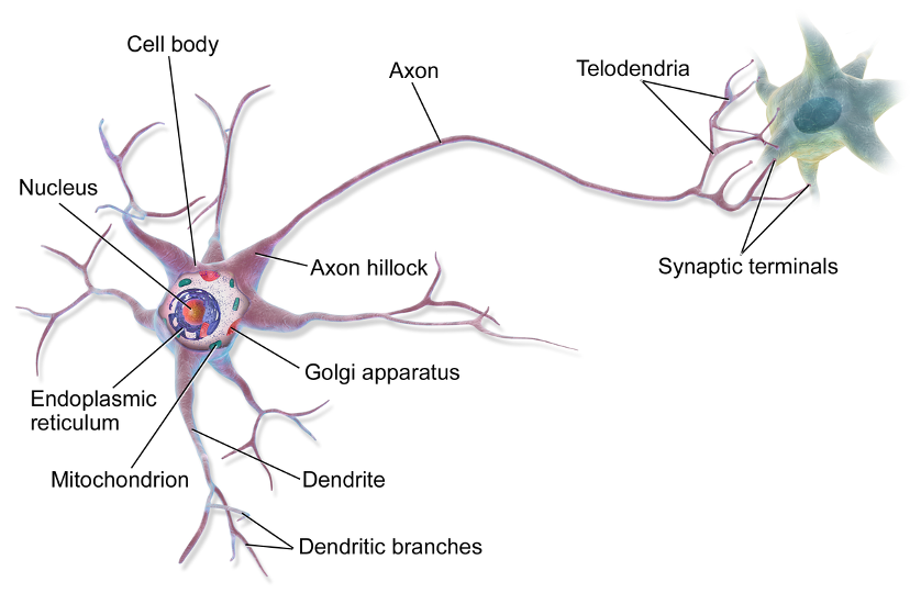
The human brain model key terms#

The idea was originally modelled on the human brain, which has ~100 billion neurons.

The soma (neuron body) holds the architecture for cell function and energy processing.
Dendrites receive information from other neurons and transfer it towards the soma.
Axons send information from the soma towards other dendrites/soma.
Dendrites and axons are connected by a synapse.

Information transfer in the human brain#

An outbound neuron produces an electrical signal called a spike that travel’s to the synapse, where chemicals called neurotransmitters.
Receptors on the inbound neuron receive the neurotransmitter, to generate another electrical signal to send the original signal to the soma.
Whether or not neurons are fired in simultaneously or in success depend on the strength/amount of the spikes. If a certain threshold is crossed, the next neuron will be activated.

neuron

Wikipedia

Are deep neural networks really like the human brain?#

Deep artificial networks were originally modelled on the human brain, and many argue for and against their likeness. See for yourself by reading the below posts!

Why deep learning?#

Deep learning is ideal for all data types, but especially text, image, video, and sound because deep representative networks store these data as large matrices. Also, error is recycled (backpropagated) to update the model weights and make better predictions during the next epoch. .

To understand deep networks, let’s start with a toy example of a single feed forward neural network - a perceptron.

Read Goodfellow et al’s Deep Learning Book to learn more: https://www.deeplearningbook.org/

import pandas as pd

# generate toy dataset
example = {'x1': [1, 0, 1, 1, 0], 
           'x2': [1, 1, 1, 1, 0], 
           'xm': [1, 0, 1, 1, 0],
           'output': ['yes', 'no', 'yes', 'yes', 'no']
           }
example_df = pd.DataFrame(data = example)
example_df

	x1	x2	xm	output
0	1	1	1	yes
1	0	1	0	no
2	1	1	1	yes
3	1	1	1	yes
4	0	0	0	no

perceptron

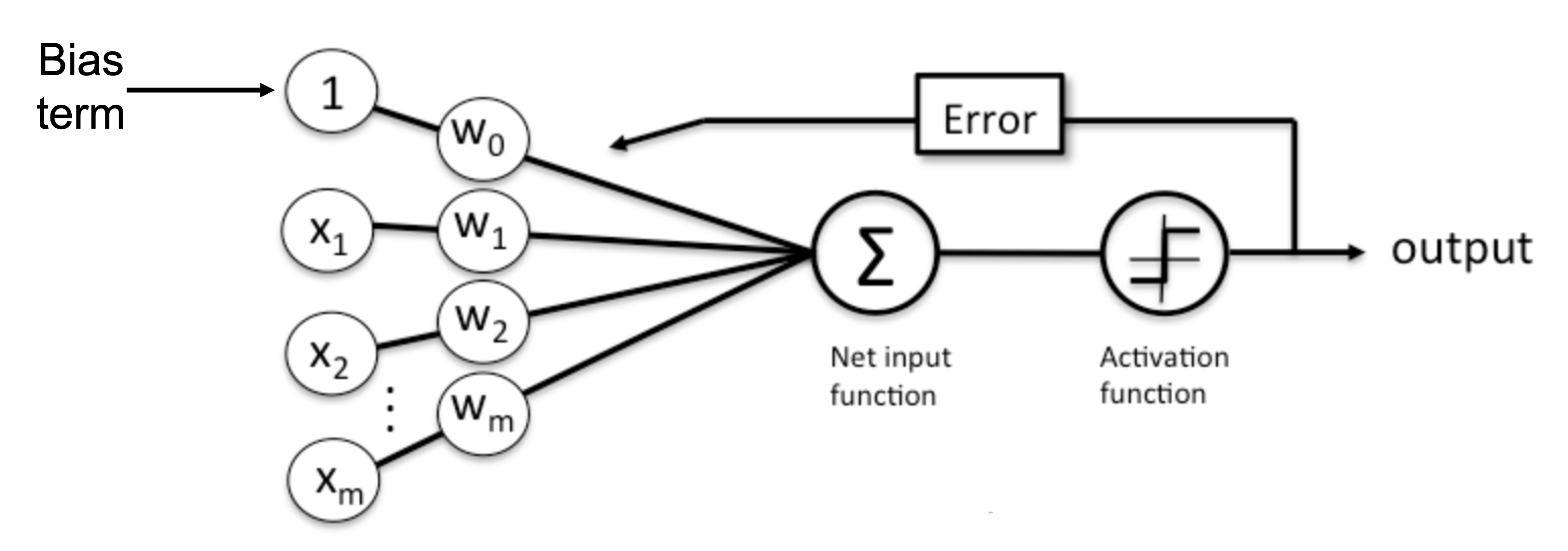
Perceptron figure modified from Sebastian Raschka’s Single-Layer Neural Networks and Gradient Descent

Perceptron key terms:

Layer: the neural architecture or the network typology of a deep learning model, usually divided into variations of input, hidden, preprocessing, encoder/decoder, and output.
Inputs/Nodes: features/covariates/predictors/independent variables (the columns of 1’s and 0s from example_df above), but they could be words from a text or pixels from an image.
Weights: the learnable parameters of a model that connect the input layer to the output via the net input (summation) and activation functions. Weights are often randomly initialized.
Bias term: A placeholder “1” assures that we do not receive only 0 predictions of our features are zero or close to 0.
Net input function: computes the weighted sum of the input layer.
Activation function: determines if a neuron should be fired or not. In binary classification for example, this defines a threshold (0.5 for example) for determining if a 1 or 0 should be predicted.
Output: a node that contains the y prediction.
Error: how far off an output prediction was. The weights are updated by adjusting the learning rate based on the error to reduce it for the next epoch.
Epoch: full pass of the training data.
Backpropagation:
Hyperparameters: our definition of the neural architecture, including but not limited to: number of hidden units, weight initialization, learning rate, batch size, dropout, etc.

What makes a network “deep”?#

A “deep” network is just network with multiple/many hidden layers for handling potential nonlinear transformations.

Fully connected layer: a layer where all nodes are connected to every node in the next layer (as indicated by the purple arrows

deep

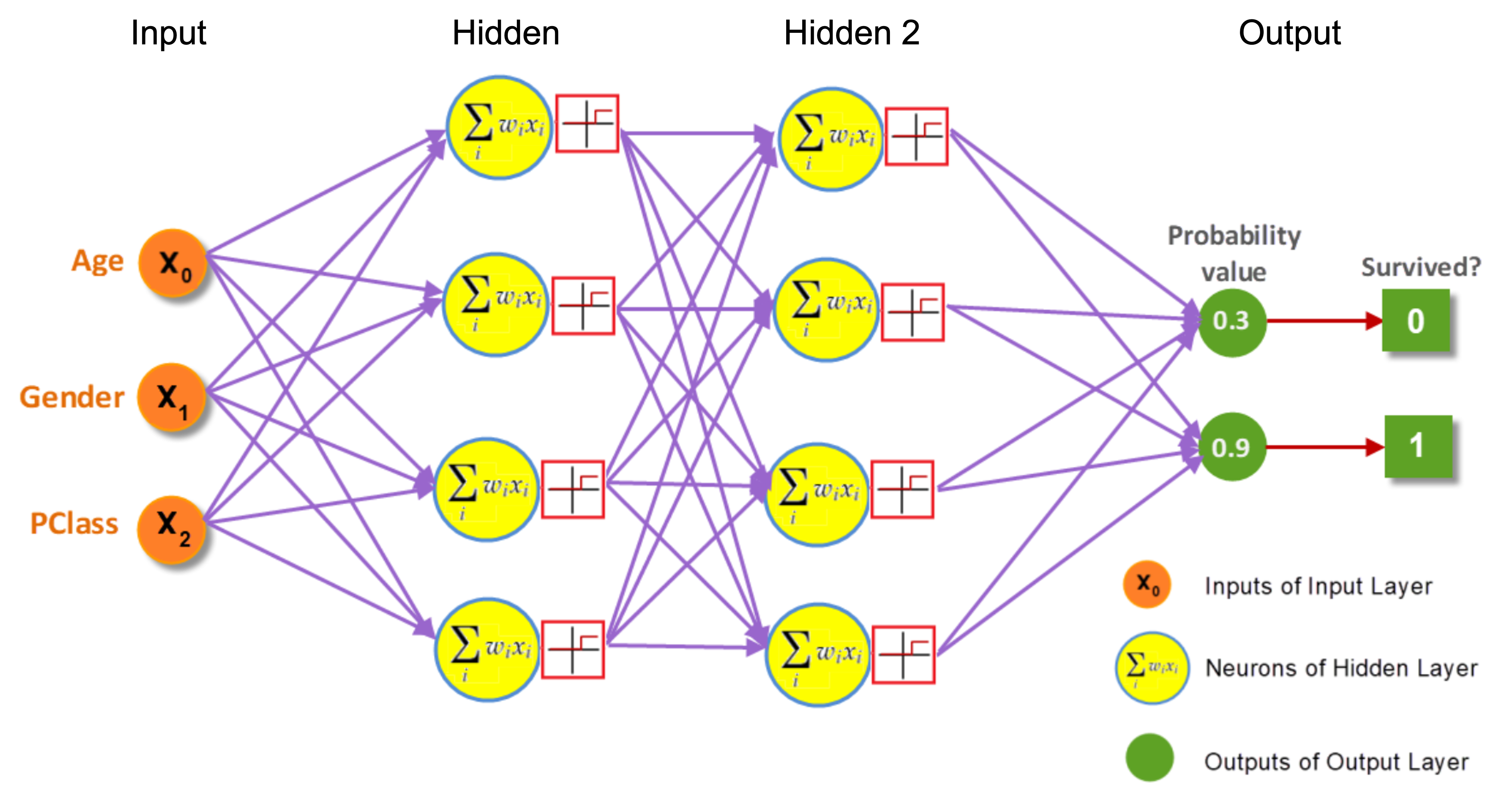
Example of “deep” network with two hidden layers modified from DevSkrol’s Artificial Neural Network Explained with an Regression Example

NOTE: Bias term not shown for some reason?

Classify images of cats and dogs#

Let’s go through François Chollet’s “Image classification from scratch” tutorial to examine this architecture and predict images of cats versus dogs.

Click here to open the Colab notebook

NOTE: One pain point for working with your own images is importing them correctly. Schedule a consultation with SSDS if you need help! https://ssds.stanford.edu/

You should also check out his deep learning book Deep Learning with Python (R version also available): https://www.manning.com/books/deep-learning-with-python-second-edition

dogcat

Text Analysis and Machine Learning (TAML) Group

Chapter 5 - Ensemble machine learning, deep learning

Contents

Chapter 5 - Ensemble machine learning, deep learning#

Ensemble machine learning#

H2O SuperLearner ensemble#

What is the Higgs Boson?#

Install h2o and Java#

Import#

Initialize an h2o cluster#

Import a sample binary outcome train/test set into H2O#

Identify predictors and response#

For binary classification, response should be a factor#

Number of CV folds (to generate level-one data for stacking)#

How to stack#

1. Generate a 2-model ensemble#

Train and cross-validate a random forest#

Random forest test set performance#

Train and cross-validate a gradient boosted machine#

Gradient boosted machine test set performance#

3. Train a stacked ensemble using the GBM and RF above#

Ensemble performance on test set#

Compare to base learner performance on the test set#

Generate predictions on a test set (if neccessary)#

4. Generate a random grid of models and stack them together#

Specify GBM hyperparameters for the grid#

5. Train a stacked ensemble using the GBM grid#

Eval ensemble performance on the test data#

6. Compare to base learner performance on the test set#

Generate predictions on a test set (if neccessary)#

Deep learning basics#

The human brain model key terms#

Information transfer in the human brain#

Are deep neural networks really like the human brain?#

Why deep learning?#

What makes a network “deep”?#

Classify images of cats and dogs#